install.packages("abd") # only if not installed (do once)Linear Regression Review
FW8051 Statistics for Ecologists
Objectives
Review important statistical concepts within the context of linear regression using simulated data:
- Sampling Distributions
- T-tests for regression coefficients
- Confidence intervals
- P-values
- How to check assumptions
Sustainable trophy hunting of African Lions
Whitman et al. 2014 Nature 428:175-178
Important to know the age of male lions to help manage trophy hunting
- Removing males over 6 has little effect on social structure
- Removing younger males is more disruptive
How, from afar, can we tell the age of a lion?
Its in the Nose!
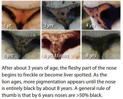
Data are contained in abd library of Program R:
Lion’s Noses
Linear Regression Assumptions
\[ Y_i = \beta_0 + \beta_1X_i + \epsilon_i \] \[ \epsilon_i \sim N(0, \sigma^2) \]
Assumptions (HILE Gauss):
- Homogeneity of variance (constant scatter about the line); \(var(\epsilon_i) = \sigma^2\)
- Independence: Correlation\((\epsilon_i, \epsilon_j) = 0\)
- Linearity: \(E[Y_i \mid X_i] = \beta_0 + X_i\beta_1\)
- Existence (we observe random variables that have finite variance; we won’t worry about this one)
- Gauss: \(\epsilon_i\) come from a Normal (Gaussian) distribution
Regression Assumptions
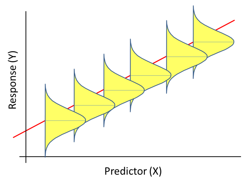
- We specify a probability distribution for \(Y_i | X_i \sim N(\mu_i, \sigma^2)\)
- We have a model for the mean \(\mu_i = \beta_0 + \beta_1X_i\)
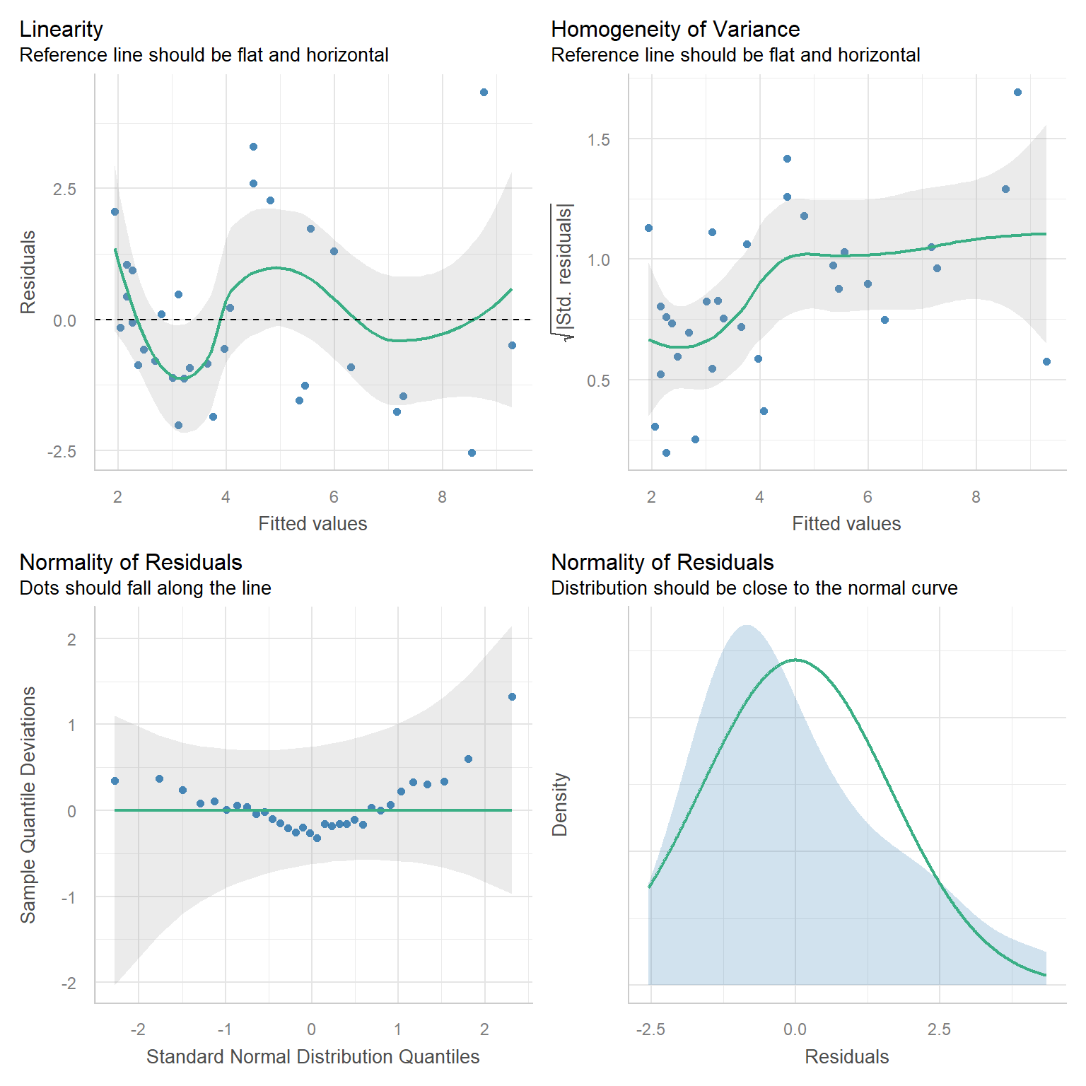
- How are these assumptions reflected in the figure? How can we evaluate the assumptions with our data?
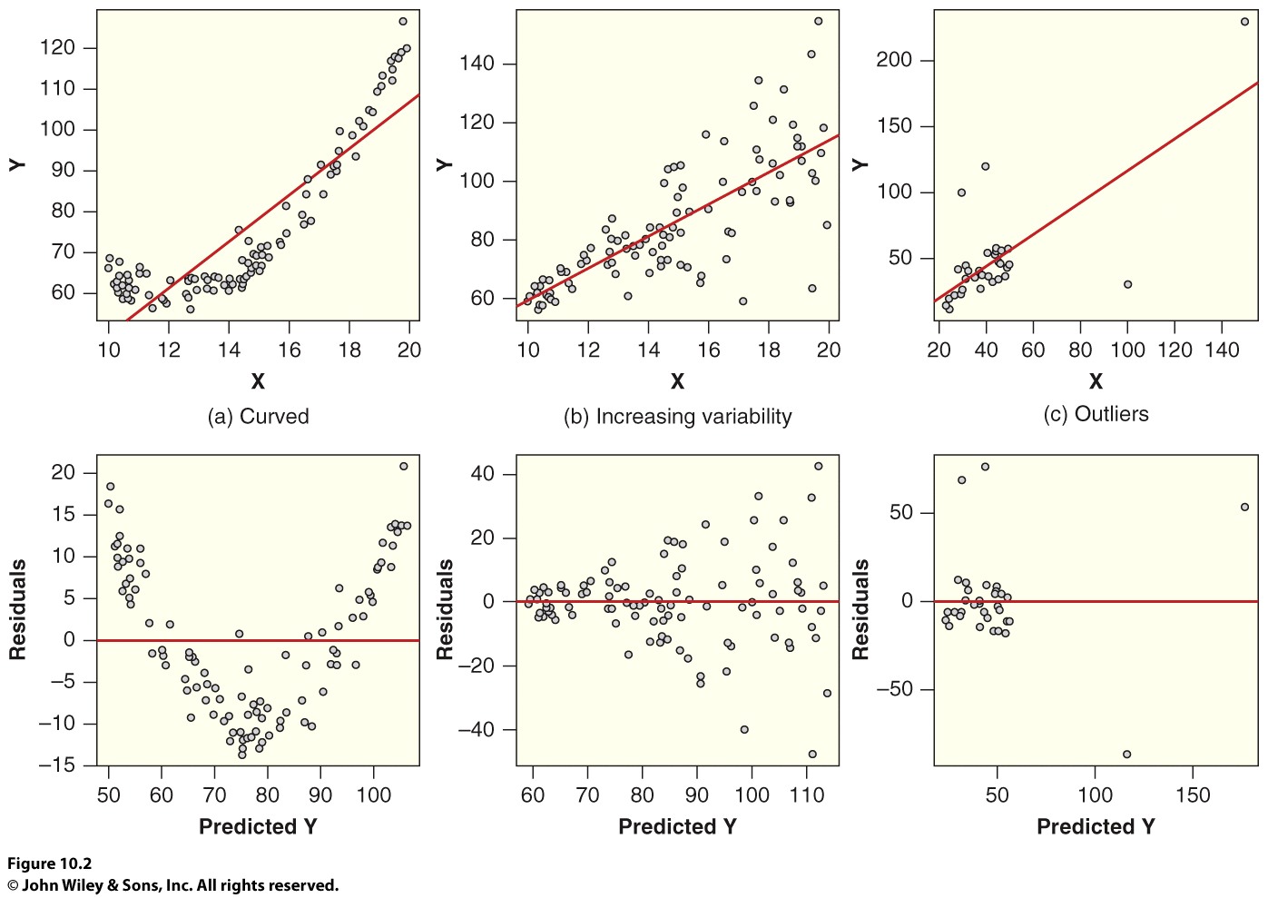
Residuals Versus Fitted
Interpretation: Intercept, Slope, t-tests and p-values, Residual Standard Error (\(\hat{\sigma}\)), \(R^2\)
Call:
lm(formula = age ~ proportion.black, data = LionNoses)

Residuals:
    Min      1Q  Median      3Q     Max
-2.5449 -1.1117 -0.5285  0.9635  4.3421

Coefficients:
                 Estimate Std. Error t value Pr(>|t|)
(Intercept)        0.8790     0.5688   1.545    0.133
proportion.black  10.6471     1.5095   7.053 7.68e-08 ***
---
Signif. codes:  0 '***' 0.001 '**' 0.01 '*' 0.05 '.' 0.1 ' ' 1

Residual standard error: 1.669 on 30 degrees of freedom
Multiple R-squared:  0.6238,    Adjusted R-squared:  0.6113
F-statistic: 49.75 on 1 and 30 DF,  p-value: 7.677e-08
Interpretation: Intercept and Slope
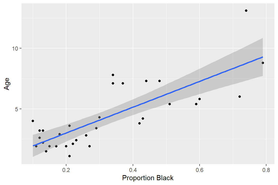
\[ \widehat{age} = 0.879 + 10.65Proportion.black \]
Intercept: Estimate of the average age of lions that have no black pigmentation on their noses (\(E[Y | X =0]\)).
Slope: Predicted change in age per unit increase in proportion black pigmentation
10.65 = \(\frac{\triangle \mbox{ age}}{\triangle \mbox{ Proportion.Black}}\)
But, proportion black < 1 for all lions.
\(\frac{\triangle age}{\triangle 0.1Proportion.Black}\) =1.065.
\(H_0: \beta_1=0\) vs. \(H_A: \beta_1 \ne 0\)?
Call:
lm(formula = age ~ proportion.black, data = LionNoses)

Residuals:
    Min      1Q  Median      3Q     Max
-2.5449 -1.1117 -0.5285  0.9635  4.3421

Coefficients:
                 Estimate Std. Error t value Pr(>|t|)
(Intercept)        0.8790     0.5688   1.545    0.133
proportion.black  10.6471     1.5095   7.053 7.68e-08 ***
---
Signif. codes:  0 '***' 0.001 '**' 0.01 '*' 0.05 '.' 0.1 ' ' 1

Residual standard error: 1.669 on 30 degrees of freedom
Multiple R-squared:  0.6238,    Adjusted R-squared:  0.6113
F-statistic: 49.75 on 1 and 30 DF,  p-value: 7.677e-08
SE, t-value, p-value
Need to understand the concept of a sampling distribution of a statistic.. . .
A sampling distribution is the distribution of sample statistics computed for different samples of the same size from the same population.
Think of many repetitions of:
- Collecting a new data set (of the same size). . .
- Calculating some statistic (\(\bar{x}\), \(\bar{x}_1-\bar{x}_2\),\(\hat{p}\), \(r\), \(\hat{\beta}\)…)
- Over and over and over…
SE \(\hat{\beta}\)
Sampling distribution of \(\hat{\beta}\) is the distribution of \(\hat{\beta}\) values across the different samples.. . .
SE = standard deviation of the sampling distribution!
Lets explore through simulation!
Simulation
Lets first generate a single data set consistent with our fitted model using the following code.
# Sample size of simulated observations
  n<-32

# Use the observed proportion.black to simulate obs.
  p.black<-LionNoses$proportion.black

# Use the estimated parameters to simulate data.
#  - can get these from the regression output
#  sigma<-summary(lm.nose)$sigma # residual variation about the line
#  betas<-coef(lm.nose) # Regression coefficients
  sigma<-1.67 # residual variation
  betas<-c(0.88, 10.65) #betas

# Create random errors (epsilons) and random responses
 epsilon<-rnorm(n,0, sigma) # Errors
 y<-betas[1] + p.black*betas[2] + epsilon # Response
Linear regression using lm function
Call:
lm(formula = y ~ p.black)

Residuals:
    Min      1Q  Median      3Q     Max
-3.2401 -0.8812 -0.3871  0.9053  3.2192

Coefficients:
            Estimate Std. Error t value Pr(>|t|)
(Intercept)   1.7028     0.5627   3.026  0.00505 **
p.black       8.9392     1.4934   5.986 1.45e-06 ***
---
Signif. codes:  0 '***' 0.001 '**' 0.01 '*' 0.05 '.' 0.1 ' ' 1

Residual standard error: 1.651 on 30 degrees of freedom
Multiple R-squared:  0.5443,    Adjusted R-squared:  0.5291
F-statistic: 35.83 on 1 and 30 DF,  p-value: 1.45e-06
In-class Exercise
Use a for loop to:
- Generate 5000 data sets using the same code
- Fit a linear regression model to each data set
- For each fit, store \(\hat{\beta}\)
This will allow us to look at the sampling distribution of \(\hat{\beta}\)!
Sampling distribution
When conducting hypothesis tests or constructing confidence intervals, we will work with the distribution of:
\[ \frac{\hat{\beta}_1-\beta_1}{\widehat{SE}(\hat{\beta}_1)} \sim t_{n-2} \]
Sampling distribution of the t-statistic
\[ \frac{\hat{\beta}_1-\beta_1}{\widehat{SE}(\hat{\beta}_1)} \sim t_{n-2} \]
Think of many repetitions of:
- Collecting a new data set (of the same size)
- Fitting the regression model
- Calculating: \(t = \frac{\hat{\beta}_1-\beta_1}{\widehat{SE}(\hat{\beta}_1)}\)
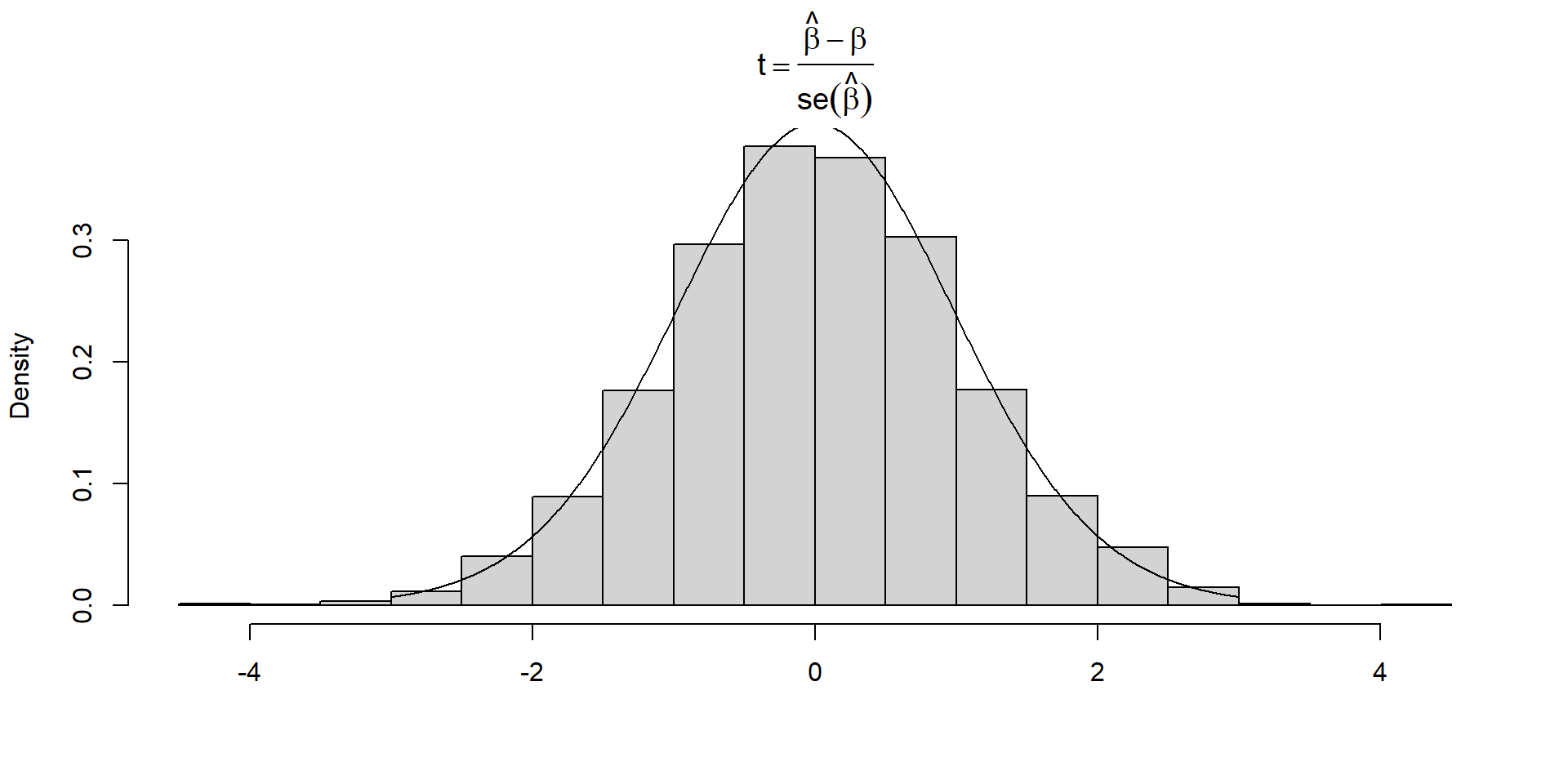
A histogram of the different t values should be well described by a Student’s t-distribution with \(n-2\) degrees of freedom.
In-class exercise
Use a for loop to:
- Generate 5000 data sets using the same code
- Fit a linear regression model to each data set
- For each fit, store \(\hat{\beta}\) and calculate: \(t = \frac{\hat{\beta}_1-\beta_1}{\widehat{SE}(\hat{\beta}_1)}\)
Helpful hints:
- \(\beta_1\) = true value used to simulate the data,
coef(lm.nose)[2]= 10.6471 - \(\hat{\beta}_1\) is extracted using:
coef(lmfit)[2] - \(\widehat{SE}(\hat{\beta}_1)\) is extracted using
sqrt(vcov(lm.temp)[2,2])
My code
nsims<-5000 # number of simulations
tsamp.dist<-matrix(NA, nsims,1) # matrix to hold results
for(i in 1:5000){
  epsilon<-rnorm(n,0,sigma) # Errors
  y<-betas[1] + betas[2]*p.black + epsilon # Response
  lm.temp<-lm(y~p.black) # lm

# Here is our statistic, calculated for each sample
  tsamp.dist[i]<-(coef(lm.temp)[2]-betas[2])/sqrt(vcov(lm.temp)[2,2])
}
# Plot results
hist(tsamp.dist, xlab="",
     main=expression(t==frac(hat(beta)-beta, se(hat(beta)))), freq=FALSE)
tvalues<-seq(-3,3, length=1000) # xvalues to evaluate t-distribution
lines(tvalues,dt(tvalues, df=30)) # overlay t-distribution
Sampling distribution of t-statistic
Confidence Interval
A confidence interval for a parameter is an interval computed from sample data by a method that will capture the parameter for a specified proportion of all samples
The confidence level specifies the proportion of samples whose intervals should contain the true parameter
The coverage rate measures the actual performance of the confidence interval proceedure and should ideally match the confidence level.
A 95% confidence interval should contain the true parameter for 95% of all samples.
Think-Pair-Share: Do the limits of the confidence interval have a sampling distribution?
Confidence Interval
\[ \frac{\hat{\beta}_1-\beta_1}{\widehat{SE}(\hat{\beta}_1)} \sim t_{n-2} \]
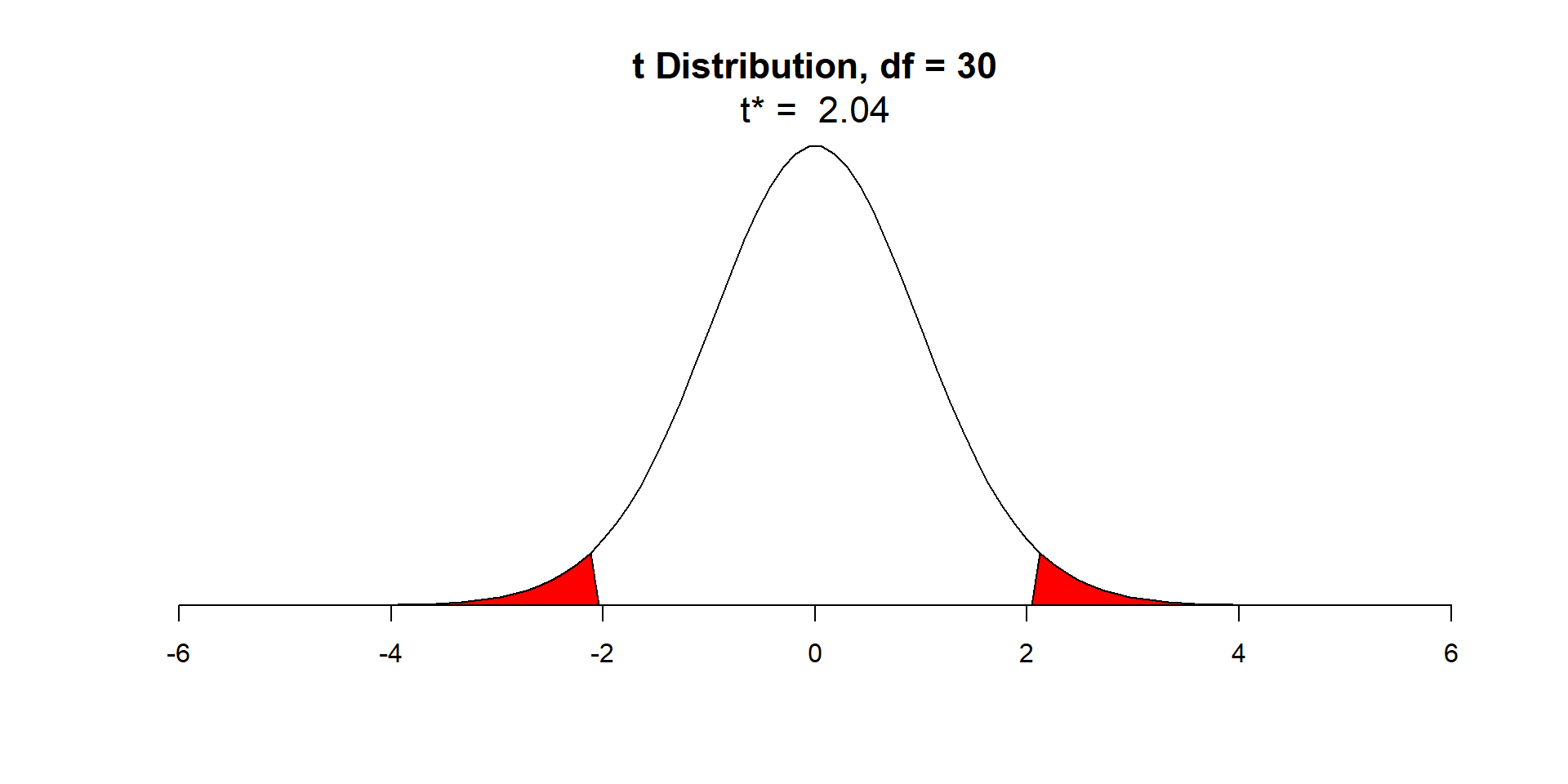
\(t_{0.025, n-2}\) = qt(p=0.025, df=30) = -\(2.04\)
\(t_{0.975, n-2}\) = qt(p=0.975, df=30) = \(2.04\)
Confidence Interval
\[ P(t_{0.025, n-2}< \frac{\hat{\beta}-\beta}{\widehat{SE}(\hat{\beta})} < t_{0.975, n-2}) = 0.95 \]
\[P(-2.04 < \frac{\hat{\beta}-\beta}{\widehat{SE}(\hat{\beta})} < 2.04) = 0.95\]
\[P(-2.04\widehat{SE}(\hat{\beta})< \hat{\beta}-\beta < 2.04\widehat{SE}(\hat{\beta})) = 0.95\]
\[P(-\hat{\beta}-2.04\widehat{SE}(\hat{\beta})< -\beta <-\hat{\beta}+ 2.04\widehat{SE}(\hat{\beta})) = 0.95\]
\[P(\hat{\beta}+ 2.04\widehat{SE}(\hat{\beta})> \beta > \hat{\beta}- 2.04\widehat{SE}(\hat{\beta})) = 0.95\]
So, take \((\hat{\beta}-2.04\widehat{SE}(\hat{\beta}),\hat{\beta}+2.04\widehat{SE}(\hat{\beta}))\) as the the 95% confidence interval.
confint function
What is wrong with the following interpretation?
\[P(7.56 \le \beta \le 13.72) = 0.95\]
- \(\beta\) is either in this particular interval (P = 1) or it is not (P = 0)
- \(P(L \le \beta \le U) = 0.95\), where \(L\) and \(U\) are random variables that determine the upper and lower limits of the 95% confidence interval
We are 95% sure that the true slope (relating proportion of nose that is black and age) falls between 7.56 and 13.73.
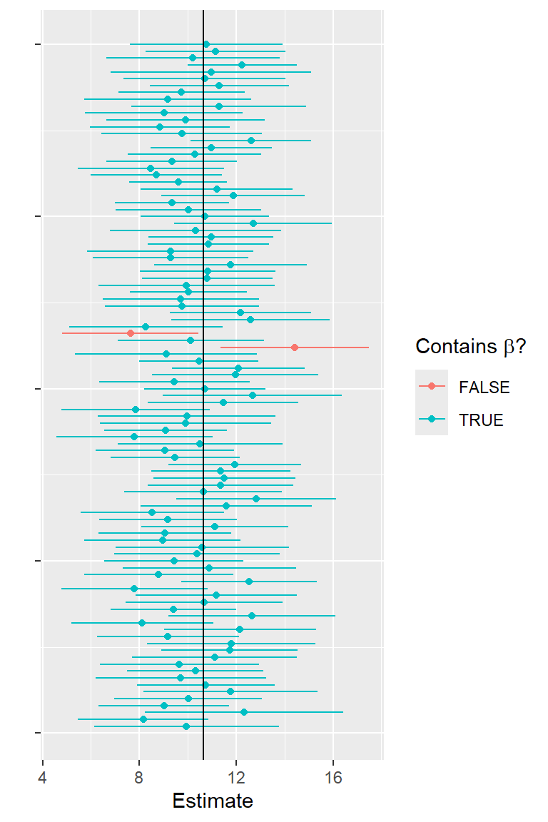
Explore CIs through simulation
Simulate another 5000 data sets in R:
Determine 95% confidence limits for each data set and examine whether or not the CI contains the true \(\beta\).
My Code
nsims<-5000 # number of simulations
Limits<-matrix(NA,nsims,2) # to hold results
beta.hats<-matrix(NA,nsims,1) # to hold estimates
for(i in 1:nsims){
  epsilon<-rnorm(n,0, sigma) # Errors
  y<-betas[1] + betas[2]*p.black + epsilon # Response
  lm.temp<-lm(y~p.black)

# Beta.hat & Confidence limits
  beta.hats[i]<-coef(lm.temp)[2]
  Limits[i,]<-confint(lm.temp)[2,]
}
# True parameter in interval?
I.in<-betas[2]>=Limits[,1] & betas[2] <= Limits[,2]

# Coverage
sum(I.in)/nsims
[1] 0.9444First 100 simulations
Hypothesis Tests
Call:
lm(formula = age ~ proportion.black, data = LionNoses)

Residuals:
    Min      1Q  Median      3Q     Max
-2.5449 -1.1117 -0.5285  0.9635  4.3421

Coefficients:
                 Estimate Std. Error t value Pr(>|t|)
(Intercept)        0.8790     0.5688   1.545    0.133
proportion.black  10.6471     1.5095   7.053 7.68e-08 ***
---
Signif. codes:  0 '***' 0.001 '**' 0.01 '*' 0.05 '.' 0.1 ' ' 1

Residual standard error: 1.669 on 30 degrees of freedom
Multiple R-squared:  0.6238,    Adjusted R-squared:  0.6113
F-statistic: 49.75 on 1 and 30 DF,  p-value: 7.677e-08
Hypothesis Tests
- State the null and alternative hypotheses
- Calculate a statistic from our data (to measure the degree to which our data deviate from what we would expect when the null hypothesis is true)
- Determine the sampling distribution of the statistic when the null hypothesis is true
- Determine the p-value = the probability of getting a statistic as extreme or more extreme as the one in step 2 when the null hypothesis is true.
The p-value measures the degree of evidence we have against the null hypothesis!
P-values
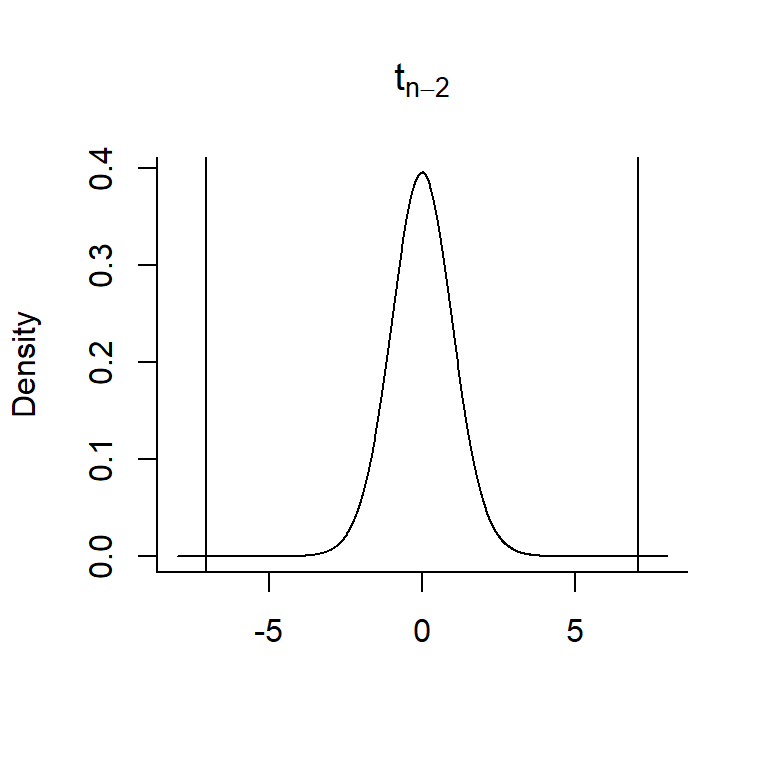
If the null hypothesis, \(H_0: \beta_1 = 0\), is true, then:
\[ t = \frac{\hat{\beta_1}-0}{\widehat{SE}({\hat{\beta_1}})} \sim t_{n-2} \]
Is the value we get for \(t = \frac{\hat{\beta_1}-0}{\widehat{SE}({\hat{\beta_1}})}\) = 7.053 consistent with \(H_0: \beta_1=0\)?
- Overlay \(t = \frac{\hat{\beta_1}-0}{\widehat{SE}({\hat{\beta_1}})}\) = 7.053 on a \(t_{n-2}\) distribution
- Determine the probability of getting a t-statistic as or more extreme as the one we observed.
Hypothesis test
- Sampling distribution when the null hypothesis is true: \[ t = \frac{\hat{\beta_1}-0}{\widehat{SE}({\hat{\beta_1}})} \sim t_{n-2} \]
- Our observed t-statistic falls in the tail of this distribution (so, the Null hypothesis is unlikely to be true!)
\(R^2\)
Call:
lm(formula = age ~ proportion.black, data = LionNoses)

Residuals:
    Min      1Q  Median      3Q     Max
-2.5449 -1.1117 -0.5285  0.9635  4.3421

Coefficients:
                 Estimate Std. Error t value Pr(>|t|)
(Intercept)        0.8790     0.5688   1.545    0.133
proportion.black  10.6471     1.5095   7.053 7.68e-08 ***
---
Signif. codes:  0 '***' 0.001 '**' 0.01 '*' 0.05 '.' 0.1 ' ' 1

Residual standard error: 1.669 on 30 degrees of freedom
Multiple R-squared:  0.6238,    Adjusted R-squared:  0.6113
F-statistic: 49.75 on 1 and 30 DF,  p-value: 7.677e-08
Sum of Squares
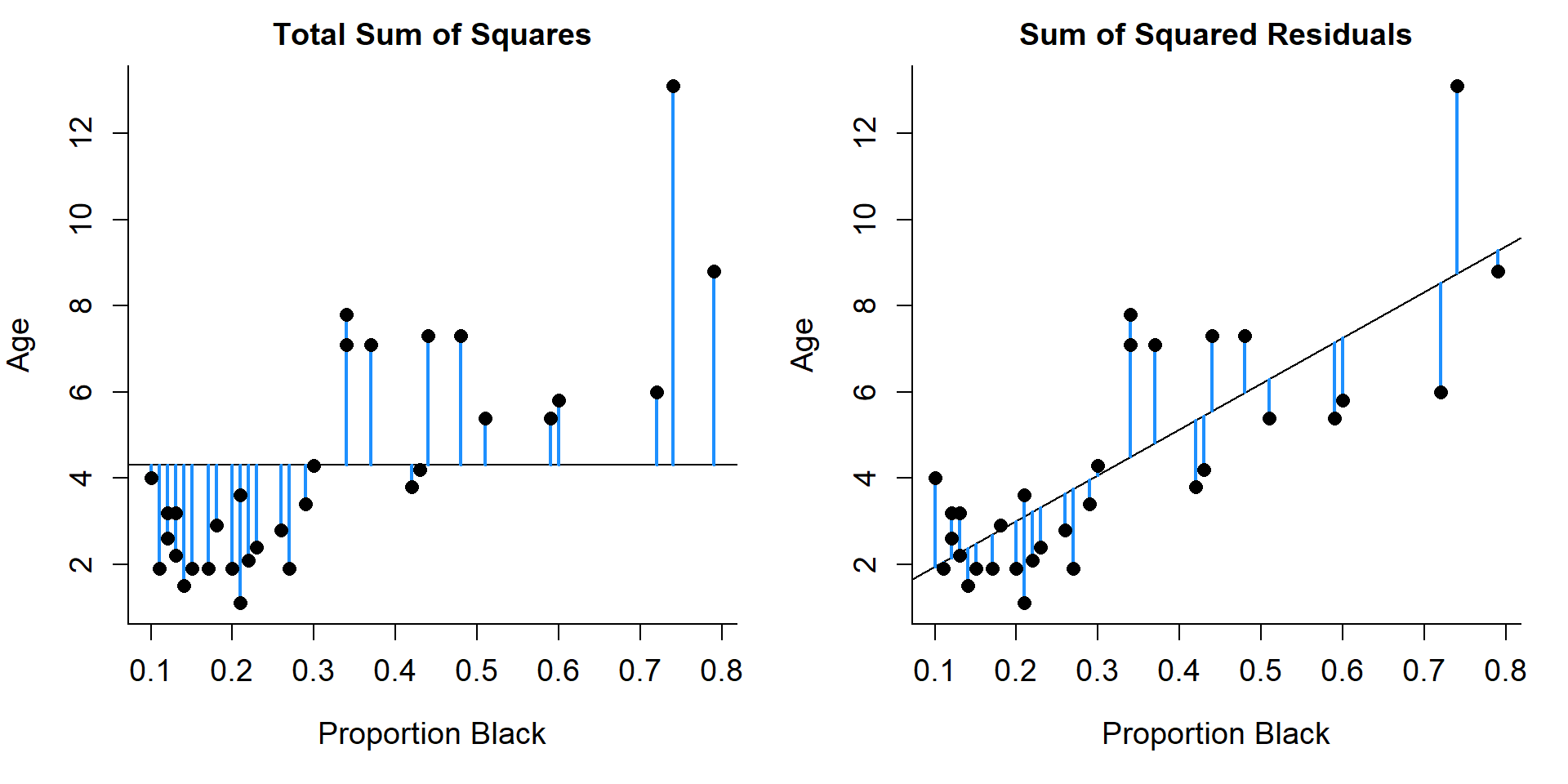
SST (Total sum of squares) = \(\sum_i^n(Y_i-\bar{Y})^2\)
SSE (Sum of Squares Error) = \(\sum_i^n(Y_i-\hat{Y})^2\)
SSR (sum of squares regression) = SST - SSE = \(\sum_i^n(\hat{Y}_i-\bar{Y})^2\)
\(R^2 = \frac{SST-SSE}{SST} = \frac{SSR}{SST}\) = proportion of the variation in our data explained by the linear model.
Residual standard error = \(\hat{\sigma}\)
- \(\sigma\) describes the amount of variability about the regression line
\(\hat{\sigma} = \sqrt{\frac{\sum_{i=1}^n(y_i-\hat{y}_i)^2}{n-p}}= \sqrt{\frac{SSE}{n-p}} = \sqrt{MSE}\). . .
- Listed as in R output from
summaryfunction. . .
- \(n-p\) since we lose one degree of freedom for each parameter we estimate
Residual Standard Error
Call:
lm(formula = age ~ proportion.black, data = LionNoses)

Residuals:
    Min      1Q  Median      3Q     Max
-2.5449 -1.1117 -0.5285  0.9635  4.3421

Coefficients:
                 Estimate Std. Error t value Pr(>|t|)
(Intercept)        0.8790     0.5688   1.545    0.133
proportion.black  10.6471     1.5095   7.053 7.68e-08 ***
---
Signif. codes:  0 '***' 0.001 '**' 0.01 '*' 0.05 '.' 0.1 ' ' 1

Residual standard error: 1.669 on 30 degrees of freedom
Multiple R-squared:  0.6238,    Adjusted R-squared:  0.6113
F-statistic: 49.75 on 1 and 30 DF,  p-value: 7.677e-08
We expect 95% of the observations to fall within 2*1.669 of the regression line.
Summary
Reviewed important statistical concepts within the context of linear regression using simulated data:
- Sampling Distributions, SEs
- T-tests for regression coefficients
- Confidence intervals
- P-values
- How to check assumptions