Confidence and Prediction Intervals

FW8051 Statistics for Ecologists

Learning Objectives

Understand the difference between a confidence interval and a prediction interval

The Lion’s Nose (from W & S)

Regression Model

\(\widehat{age} = 0.879 + 10.65\)Proportion.black

summary(lm.nose)

Call:
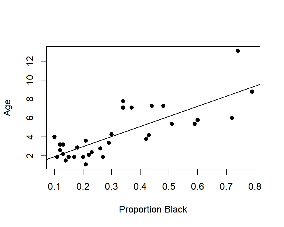
lm(formula = age ~ proportion.black, data = LionNoses)

Residuals:
    Min      1Q  Median      3Q     Max 
-2.5449 -1.1117 -0.5285  0.9635  4.3421 

Coefficients:
                 Estimate Std. Error t value Pr(>|t|)    
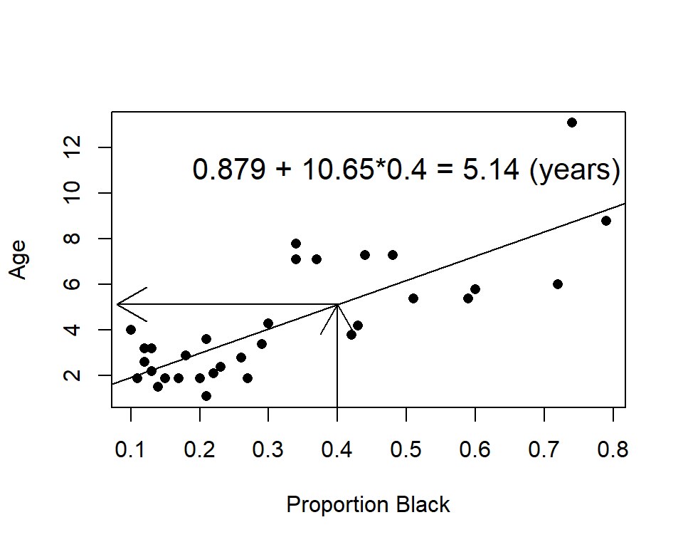
(Intercept)        0.8790     0.5688   1.545    0.133    
proportion.black  10.6471     1.5095   7.053 7.68e-08 ***
---
Signif. codes:  0 '***' 0.001 '**' 0.01 '*' 0.05 '.' 0.1 ' ' 1

Residual standard error: 1.669 on 30 degrees of freedom
Multiple R-squared:  0.6238,    Adjusted R-squared:  0.6113 
F-statistic: 49.75 on 1 and 30 DF,  p-value: 7.677e-08

Predictions

If we see a lion with a nose that is 40% black, what age would we predict?

Predictions

If we see a lion with a nose that is 40% black, what age would we predict?

Predictions

If we see a lion with a nose that is 40% black, what age would we predict?

Inference for Regression Predictions

For a single predictor model and a particular value (\(X=x\)) of the predictor, the predicted response (\(Y\)) is given by:

\(\hat{y} = \beta_0 + \beta_1x\)

How accurate is the prediction?

Two types of intervals:

• Confidence Interval for Mean \(Y\) (at \(X=x\))
• Prediction Interval for Individual \(Y\)’s (at \(X=x\))

What’s the Difference? [Think-Pair-Share]

Confidence versus prediction interval

Goal: 95% sure we capture the average age of lions with noses that are 40% black:

\(\Rightarrow\) Confidence interval for the mean \(Y\)

Goal: 95% sure we capture the age of an individual lion with a 40% black nose:

\(\Rightarrow\) Prediction interval for individual \(Y\)

Intervals

• A confidence interval has a given chance of capturing the mean \(y\) value at a specified \(x\) value

• A prediction interval has a given chance of capturing the \(y\) value for a particular case at a specified \(x\) value

• For a given \(x\) value, which will be wider?

• Confidence interval

• Prediction interval

A confidence interval only addresses uncertainty about the line, a prediction interval also includes the scatter of the points around the line

CI and PI for Regression

CI for the mean \(Y\) tries to capture the “true” line for the population.

PI for individual \(Y\)’s tries to capture the data points in the population.

Lets start by considering how much the fitted line might vary from sample to sample. How can we explore this question?

Bootstrap!

Lets fit 1000 lines to bootstrap samples

nboots<-1000
betas<-matrix(NA, nboots,2)
nobs<-nrow(LionNoses)
for(i in 1:nboots){
  bootdat<-LionNoses[sample(1:nobs, nobs,replace=T),]
  lmfit<-lm(age~proportion.black, data=bootdat)
  betas[i,]<-coef(lmfit)
}

Now, lets plot them!

with(LionNoses,plot(proportion.black,age,  xlab="Proportion Black", ylab="Age", pch=16))
lm.nose<-lm(age~proportion.black, data=LionNoses)
abline(lm.nose) # best fit line, now add bootstrap lines (below)
for(i in 1:1000){abline(a=betas[i,1],b=betas[i,2], col=rgb(0.8,0,0, alpha=0.05))}

Middle 95% of predicted values gives the CI for the mean age when proportion black is 0.40.

Using R: predict function

(CI.boot <- quantile(phats, prob=c(0.025, 0.975))) # Bootstrap CI

    2.5%    97.5% 
4.395015 5.952447 

If we want to relax the normality assumption: We are 95% sure that the mean age of lions with noses that are 40% black is between 4.4 and 5.95.

newdata<-data.frame(proportion.black=0.4)
predict(lm.nose, newdata, interval="confidence")

       fit      lwr      upr
1 5.137854 4.489386 5.786322

If we believe our assumptions (HILG): We are 95% sure that the mean age of lions with noses that are 40% black is between 4.49 and 5.79.

Confidence Interval for mean \(Y\) at each \(X\)

newdata<-data.frame(proportion.black=seq(0.08, 0.81, length=100))
predict.mean<-as.data.frame(predict(lm.nose, newdata, interval="confidence"))
with(LionNoses,plot(proportion.black,age,  xlab="Proportion Black", ylab="Age", pch=16))
abline(lm.nose)
lines(newdata$proportion.black, predict.mean$lwr, lty=2)
lines(newdata$proportion.black, predict.mean$upr, lty=2)

Confidence Interval

• Captures uncertainty regarding the “true” population line
• Does NOT capture uncertainty in individual data values
• CI gets wider for more extreme predictor values

We find a lion that has a nose that is 40% black, and we estimate its age. Can we construct an interval that will contain this animal’s true age 95% of the time?

Prediction Interval for Individual \(Y\)

Need to account for the random variability (error) around the line.

Remember: \(\epsilon \sim N(0, \sigma^2)\). \(\hat{\sigma} = s_{\epsilon} = \sqrt{\sum_{i=1}^n{\frac{(y_i-\hat{y}_i)^2}{n-2}}}\)

Prediction Intervals in R:

predict.ind<-as.data.frame(predict(lm.nose, newdata, interval="prediction"))
with(LionNoses,plot(proportion.black,age,  xlab="Proportion Black", ylab="Age", pch=16))
abline(lm.nose)
lines(newdata$proportion.black, predict.ind$lwr, lty=2)
lines(newdata$proportion.black, predict.ind$upr, lty=2)

Captures 31/32 = 96% of the data values.

CI and PI

with(LionNoses,plot(proportion.black,age,  xlab="Proportion Black", ylab="Age", pch=16))
abline(lm.nose)
lines(newdata$proportion.black, predict.mean$lwr, lty=2, col="red", lwd=2)
lines(newdata$proportion.black, predict.mean$upr, lty=2, col="red", lwd=2)
lines(newdata$proportion.black, predict.ind$lwr, lty=2)
lines(newdata$proportion.black, predict.ind$upr, lty=2)
legend(0.08, 13, lty=2, col=c("black", "red"), c("Prediction", "Confidence"), bty="n", cex=1.4)

Two forms of intervals for regression predictions:

• CI for mean Y at a particular \(x\)
• PI for individual Y’s at a particular \(x\)