Bootstrapping

FW8051 Statistics for Ecologists

Objectives

  • To understand how a bootstrap can be used to quantify uncertainty, particularly when assumptions of linear regression may not be met.
  • To further your coding skills by implementing a cluster-level bootstrap appropriate for certain types of data sets containing repeated observations.

RIKZ data

Abundances from \(\sim\) 75 invertebrate species measured on various beaches along Dutch Coast collected by the Dutch governmental institute.

Map of Netherlands

Selected from: Zuur, A. F., E. N. Ieno, and G. M. Smith. 2009. Analyzing Ecological Data. Springer, New York.

RIKZ data

Sampling Effort:

  • 9 beaches (high, medium, low exposure)

  • 5 stations at each beach.

Variables:

  • Richness = species richness (number of species counted).

  • NAP = height of the sample site (relative to sea level).

    • Lower values imply more time spent under water.

    • Higher values typically found further up the beach.

Gerard Janssen, RIKZ

Picture of Gerard janssen and his crew sampling on the beach

Picture of Gerard janssen and his crew sampling on the beach

\(\hat{Y}_i=6.886-2.867X_i+E_i\)

Scatterplot of species richness versus NAP

Regression Output

 lmfit.R<-lm(Richness~NAP, data=RIKZdat)
 summary(lmfit.R)

Call:
lm(formula = Richness ~ NAP, data = RIKZdat)

Residuals:
    Min      1Q  Median      3Q     Max 
-5.0675 -2.7607 -0.8029  1.3534 13.8723 

Coefficients:
            Estimate Std. Error t value Pr(>|t|)    
(Intercept)   6.6857     0.6578  10.164 5.25e-13 ***
NAP          -2.8669     0.6307  -4.545 4.42e-05 ***
---
Signif. codes:  0 '***' 0.001 '**' 0.01 '*' 0.05 '.' 0.1 ' ' 1

Residual standard error: 4.16 on 43 degrees of freedom
Multiple R-squared:  0.3245,    Adjusted R-squared:  0.3088 
F-statistic: 20.66 on 1 and 43 DF,  p-value: 4.418e-05

Model for the Data

\(Y_i = \beta_0 + \beta_1X_i + \epsilon_i\)

\(\epsilon_i \sim N(0, \sigma^2)\)

\(Y_i \sim N(\mu_i, \sigma^2)\) \(\mu_i = \beta_0 + \beta_1X_i\)

3-dimensional plot showing Richness versus NAP with normal distribution plotted in third dimension.

Linear Regression

Assumptions (HILE Gauss):

  • Homogeneity of variance (constant scatter about the line); \(var(\epsilon_i) = \sigma^2\)
  • Independence: Correlation\((\epsilon_i, \epsilon_j) = 0\)
  • Linearity: \(E[Y_i \mid X_i] = \beta_0 + X_i\beta_1\)
  • Existence (we observe random variables that have finite variance)
  • Gauss: \(\epsilon_i\) come from a Normal (Gaussian) distribution

Assumptions

performance::check_model(lmfit.R, 
   check = c("linearity", "homogeneity", "qq", "normality"))
Residual plots for the linear regression model.

Linearity?

Scatterplot of species richness versus NAP

\(Richness_i=6.886-2.867*NAP_i+\epsilon_i\)

What if NAP \(>\) 2.3?

Independence

Are 2 observations from the same beach more alike than 2 observations from 2 different beaches (after accounting for NAP)?

Consequence? SE’s for \(\hat{\beta}\) too small?

Alternatives

  • Transformations (constant variance, Normality, linearity)
    • log(Richess) = \(\beta_0 + \beta_1NAP\) ?
  • Add other variables (can help if patterns in residuals or non-constant variance)?
  • Can model mean and variance using “Generalized least squares” (gls) (Ch 4 of Zuur et al.)

\[Y_i \sim N(\mu_i, \sigma^2_i)\] \[\mu_i = \beta_0 + X_i\beta\] \[\sigma^2_i = f(X_i; \theta)\]

  • Use generalized linear models for count data (naturally allows the variance to increase with the mean)

  • Bootstrap (to deal with non-constant variance, clustering)

Assumptions

Linear regression relies on least-squares:

\(\hat{\beta}\) minimizes: \(\sum_{i=1}^{n}(Y_i-[\beta_0+ X_i\beta_1])^2\).


Normality is needed for inference, i.e., ensures the sampling distribution of \(\frac{\hat{\beta}-\beta}{\widehat{SE}(\hat{\beta})} \sim t_{n-p}\)


To relax these assumptions, we will consider using a bootstrap for inference.

Illustration of a sampling distribution

Illustration of a sampling distribution

Illustration of a sampling distribution

Illustration of a sampling distribution

Illustration of a sampling distribution

Illustration of a sampling distribution

Illustration of a sampling distribution

Illustration of a sampling distribution

If assumptions hold, we know the sampling distribution!

\(\frac{\hat{\beta}-\beta}{SE(\hat{\beta})} \sim t_{n-2}\)

Reality

We only have 1 sample, what do we do?

BOOTSTRAP

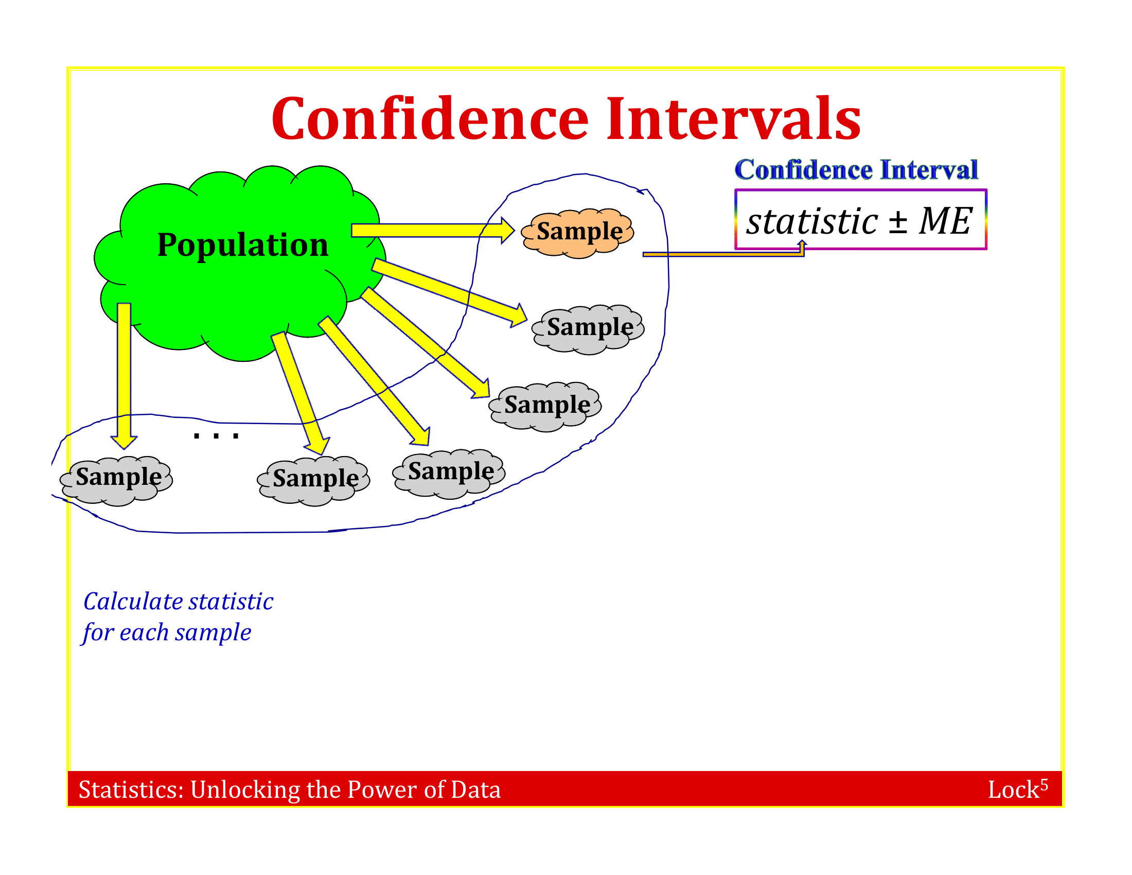
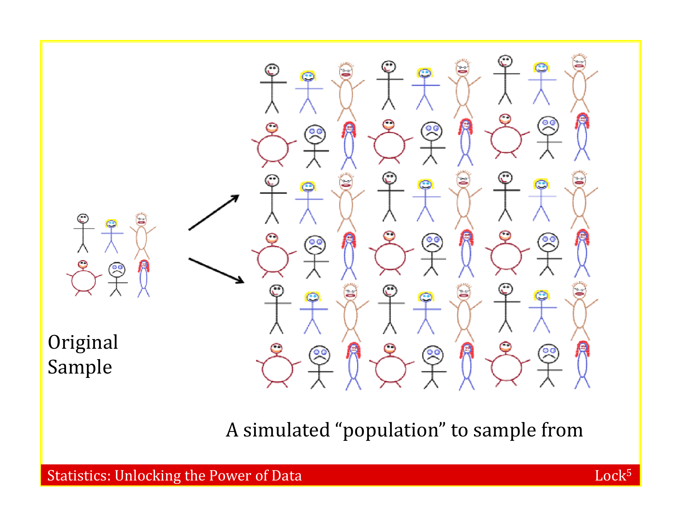
  • Imagine the “population” is many, many copies of the original sample
  • Resample this population many times and fit the model to each data set

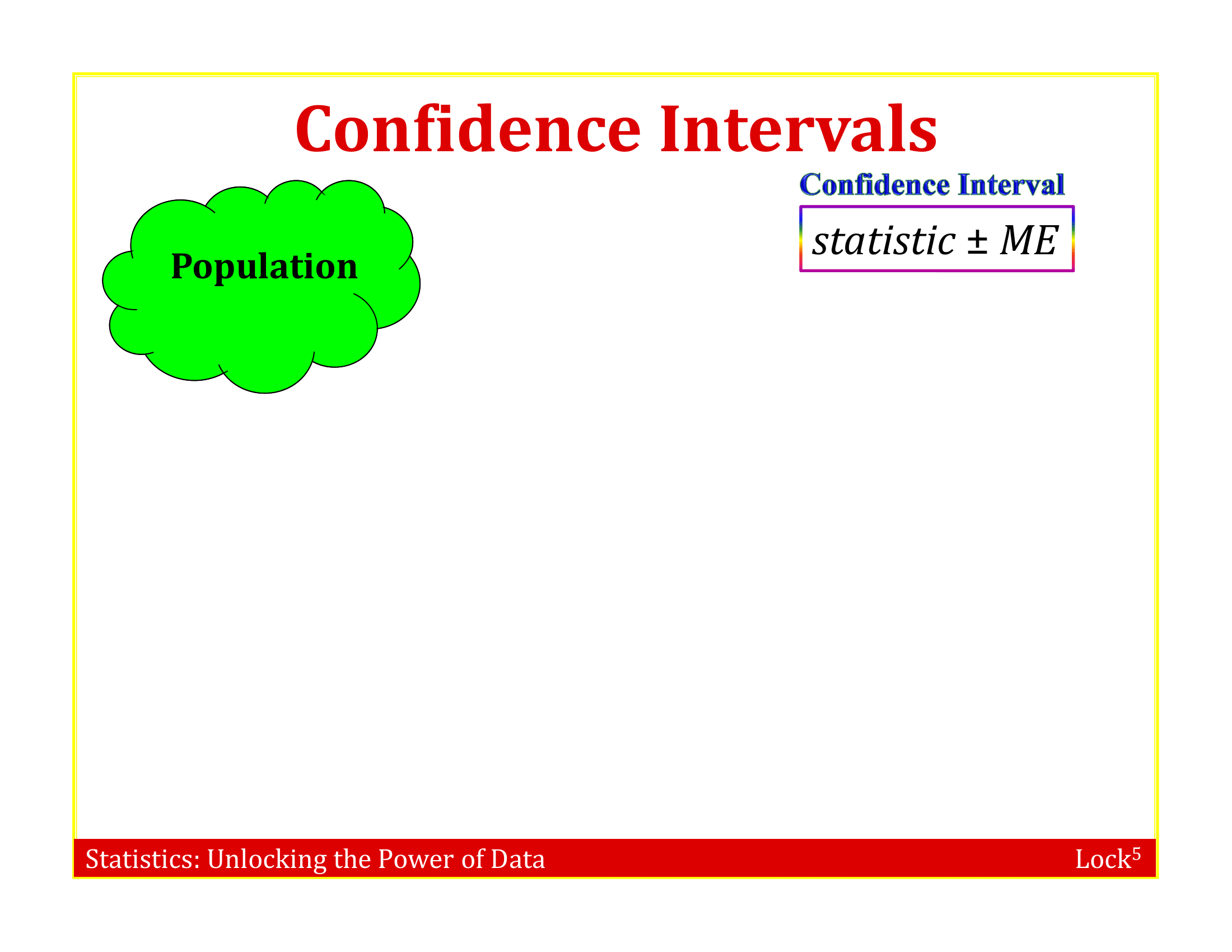
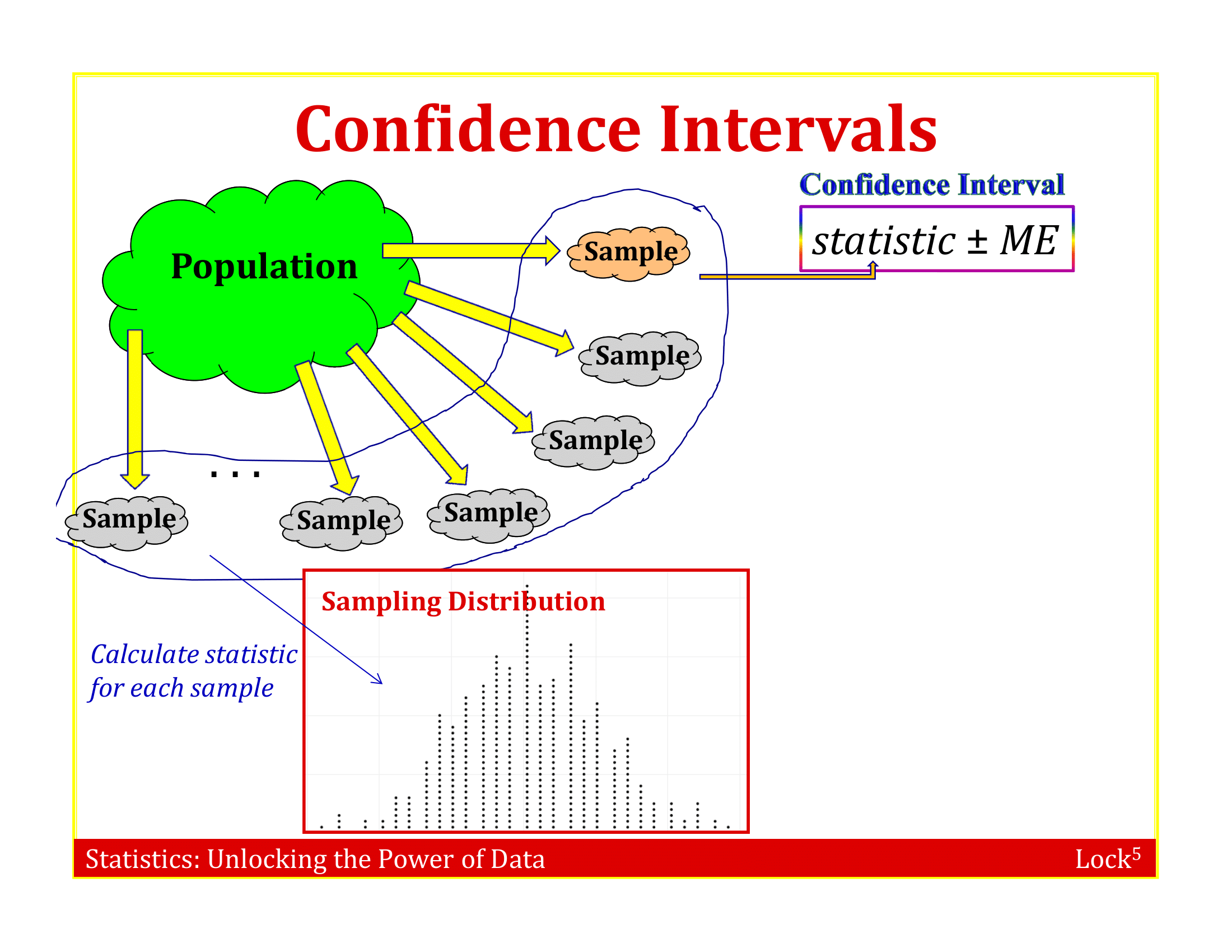
What do you have to assume?

  • The sample is representative of the population (otherwise, its pointless to try to generalize from sample to population)

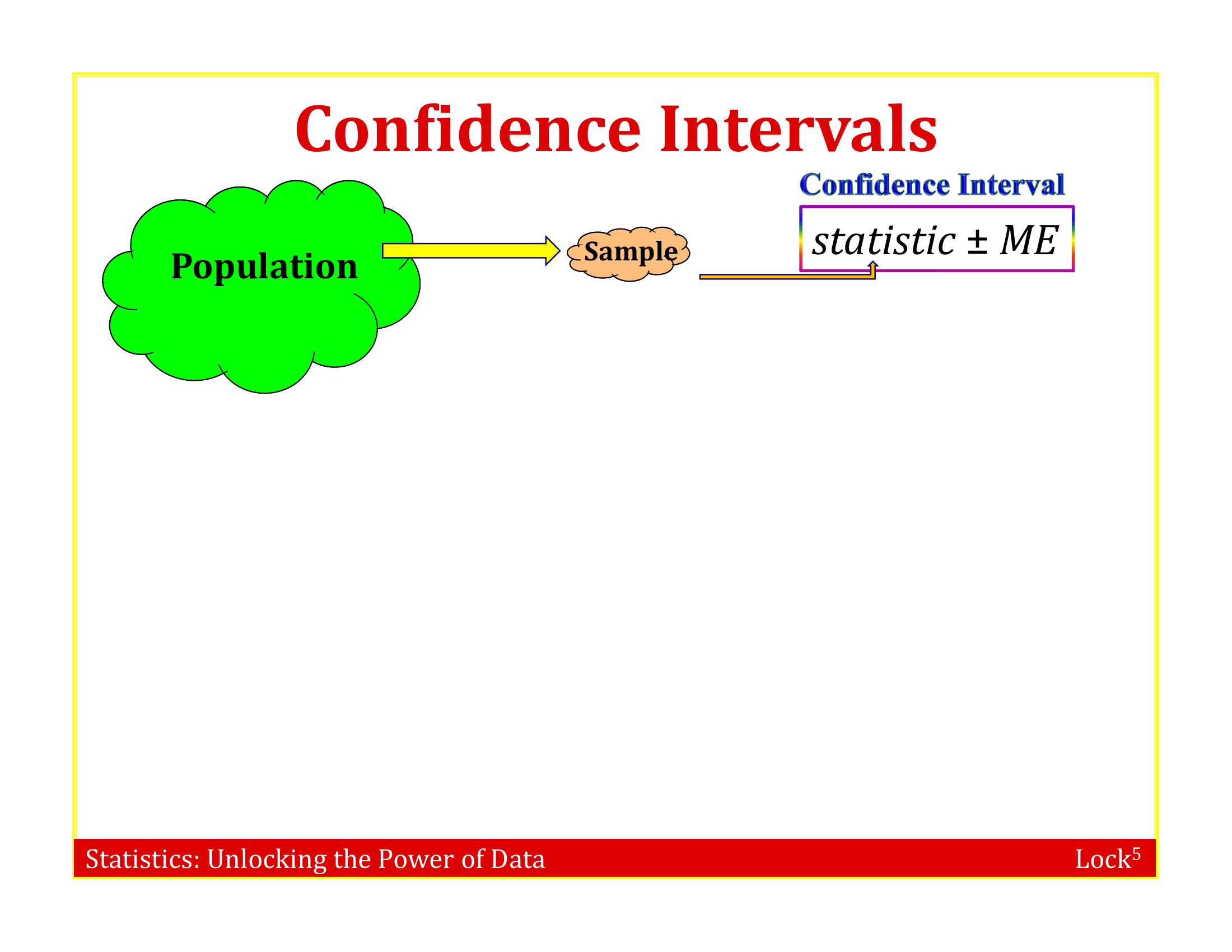
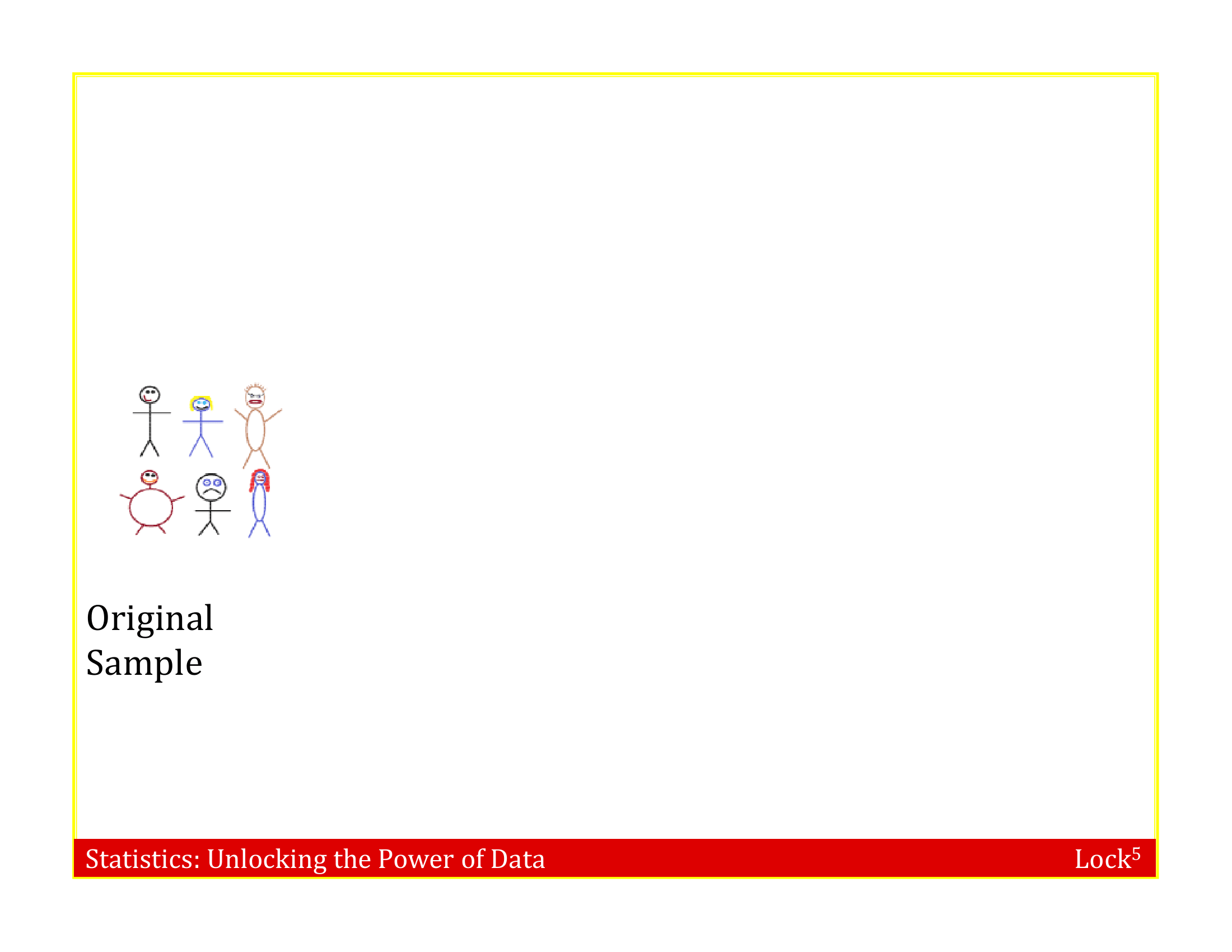
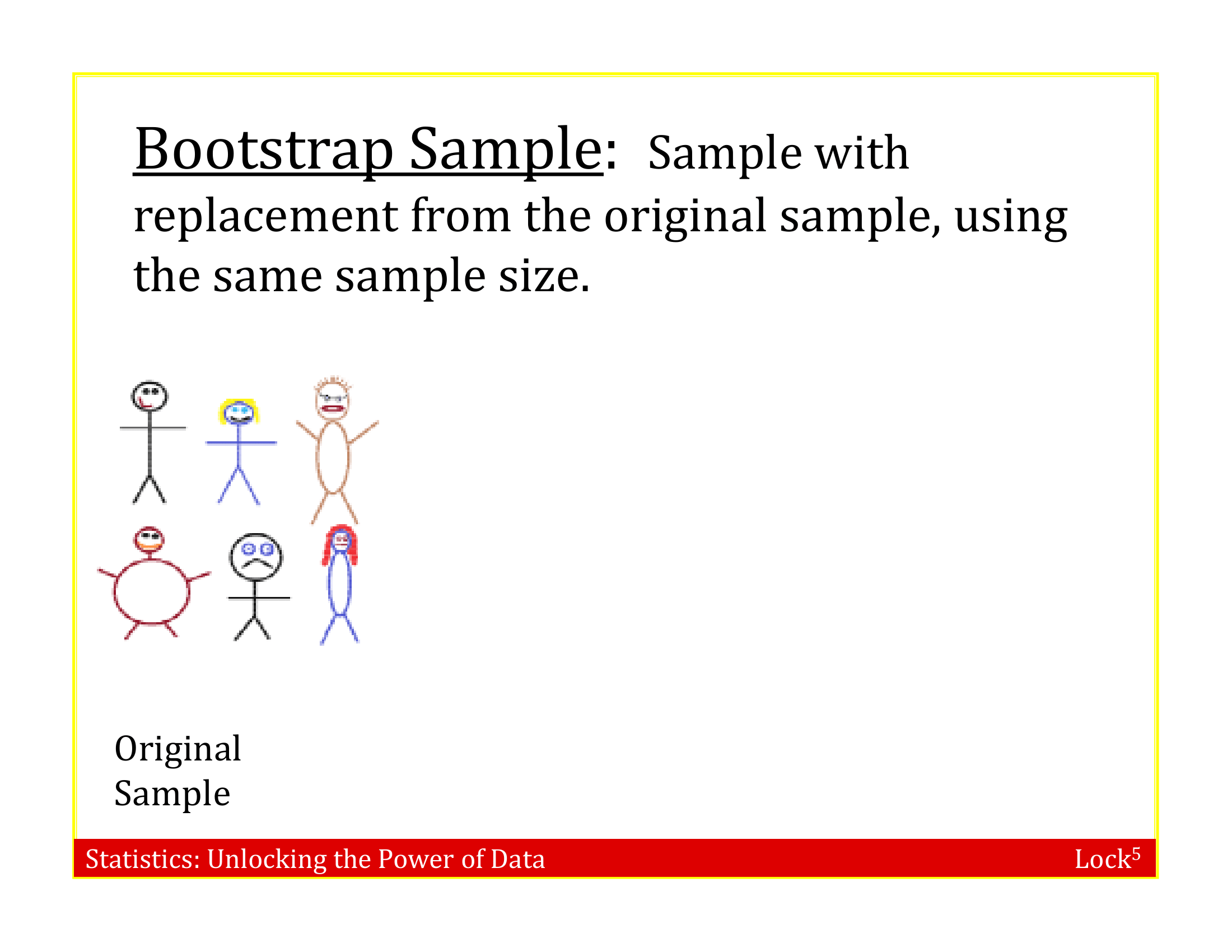
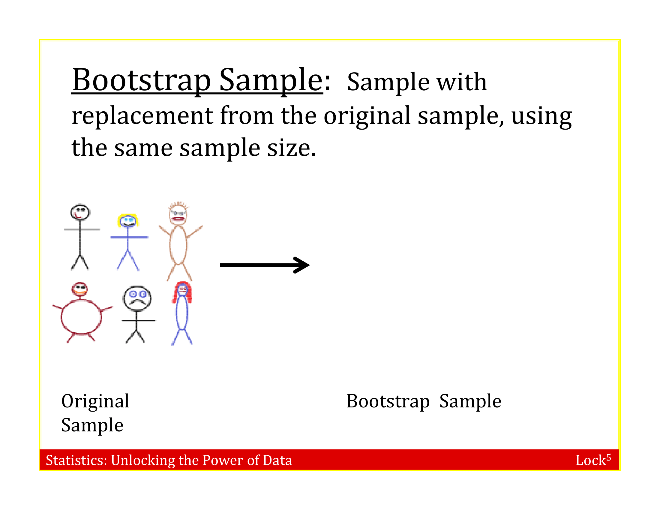
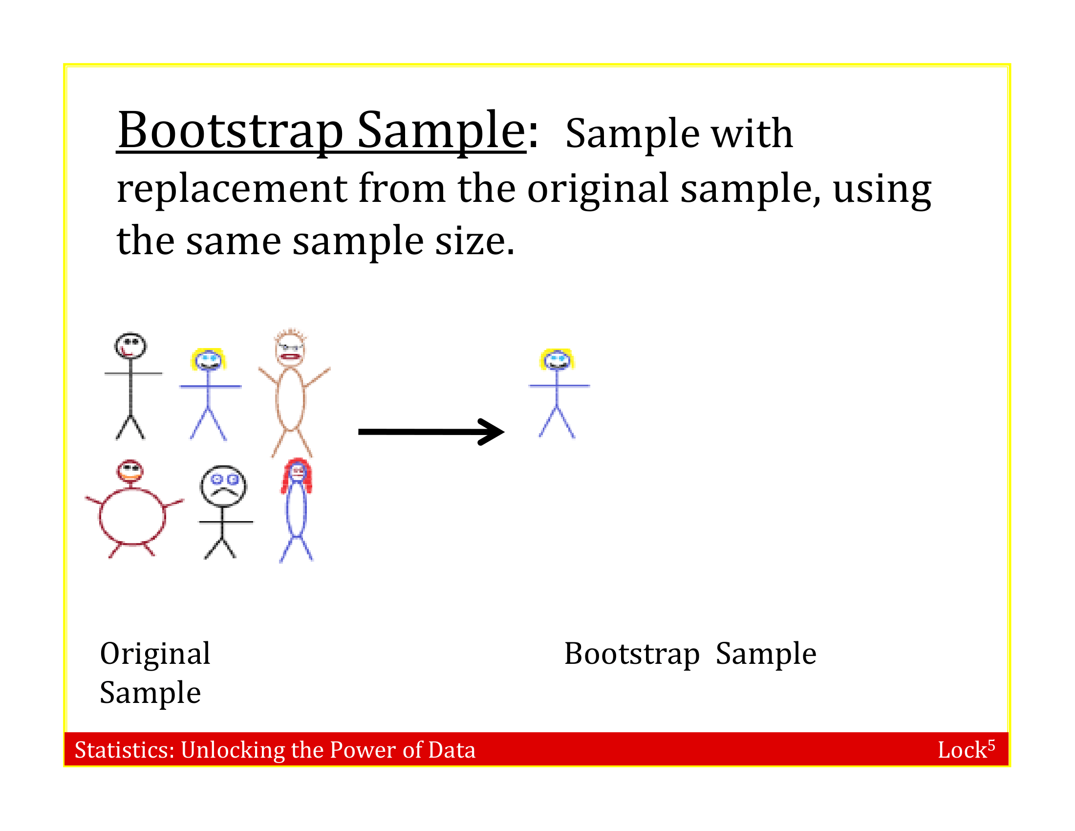
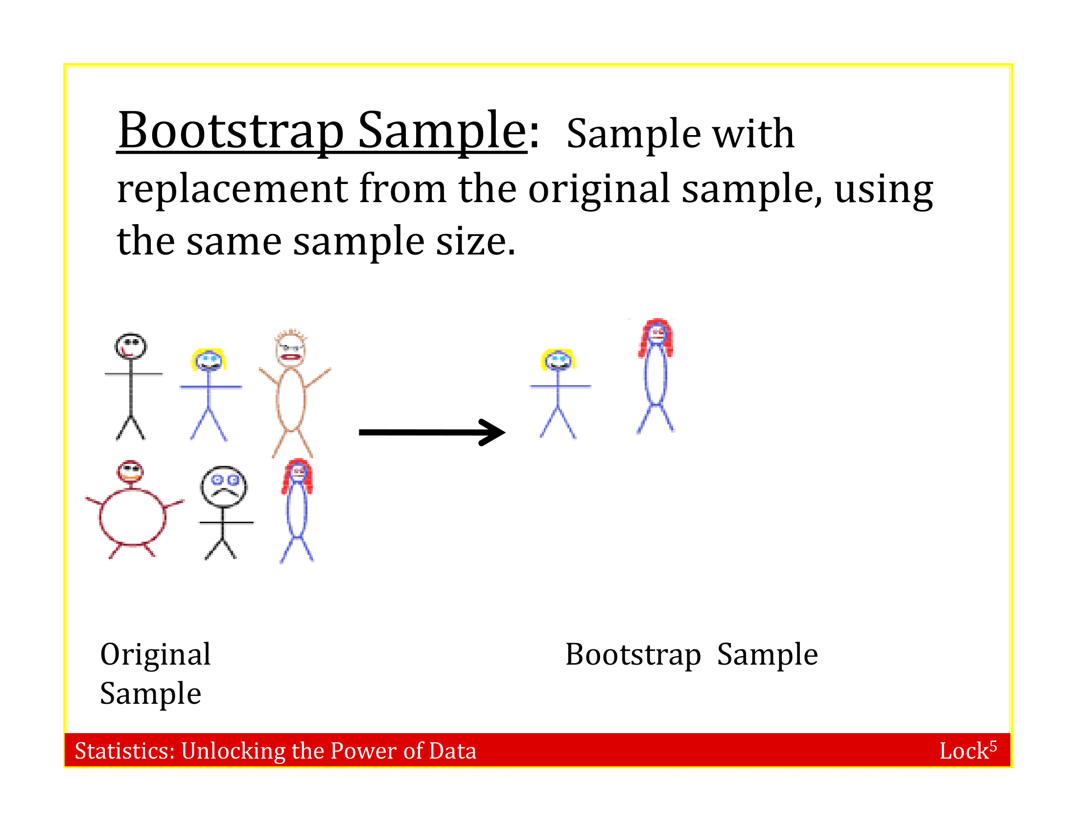
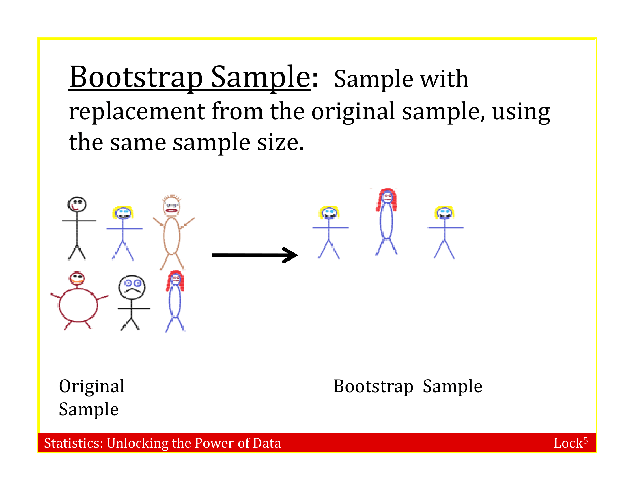
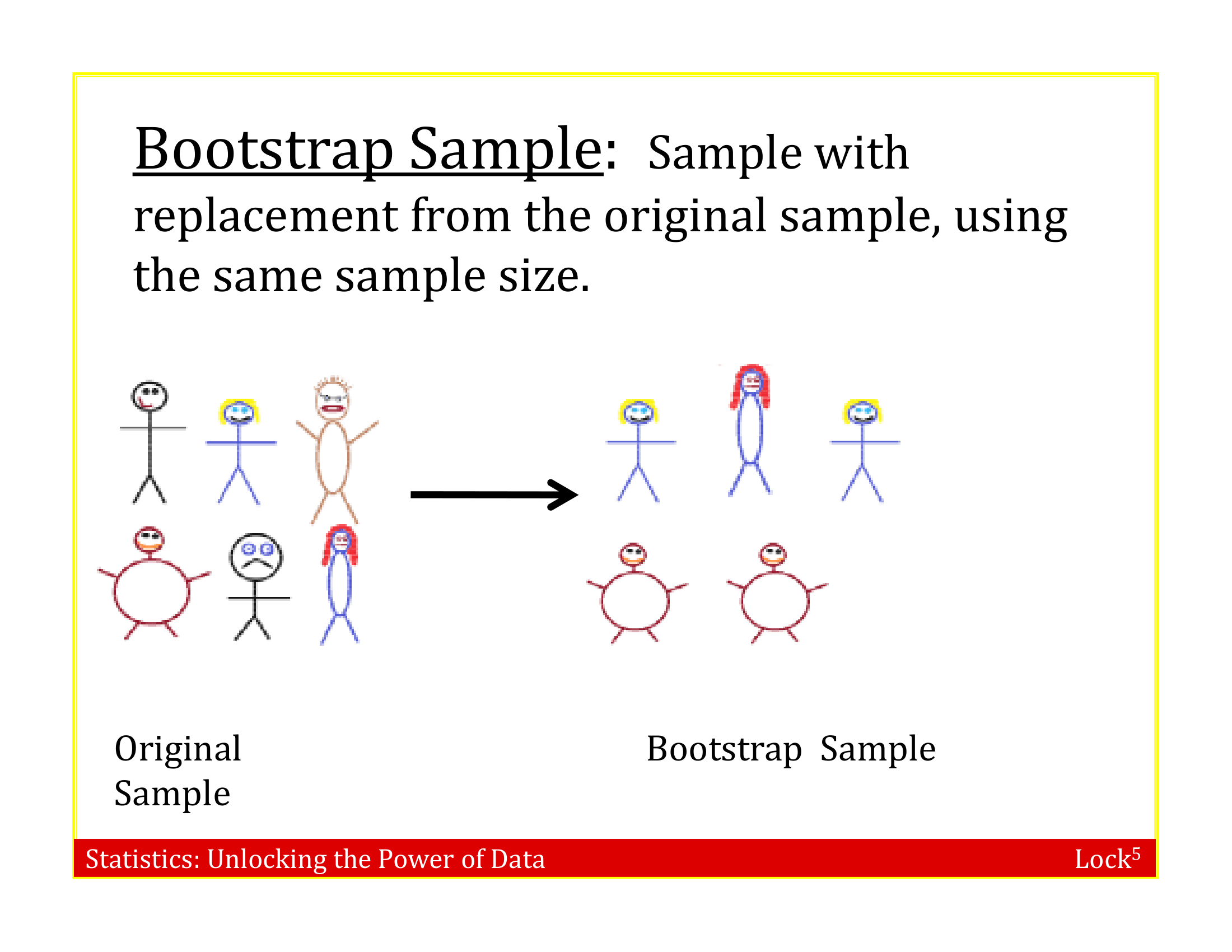
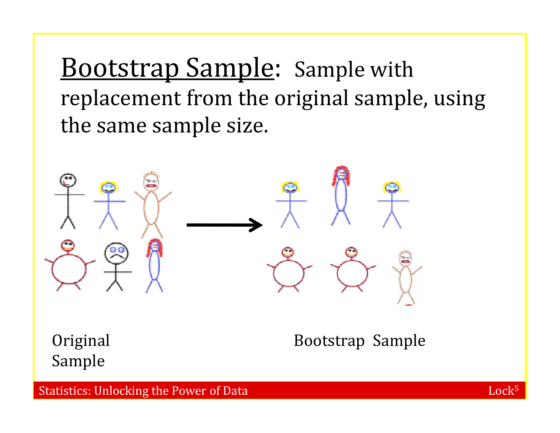
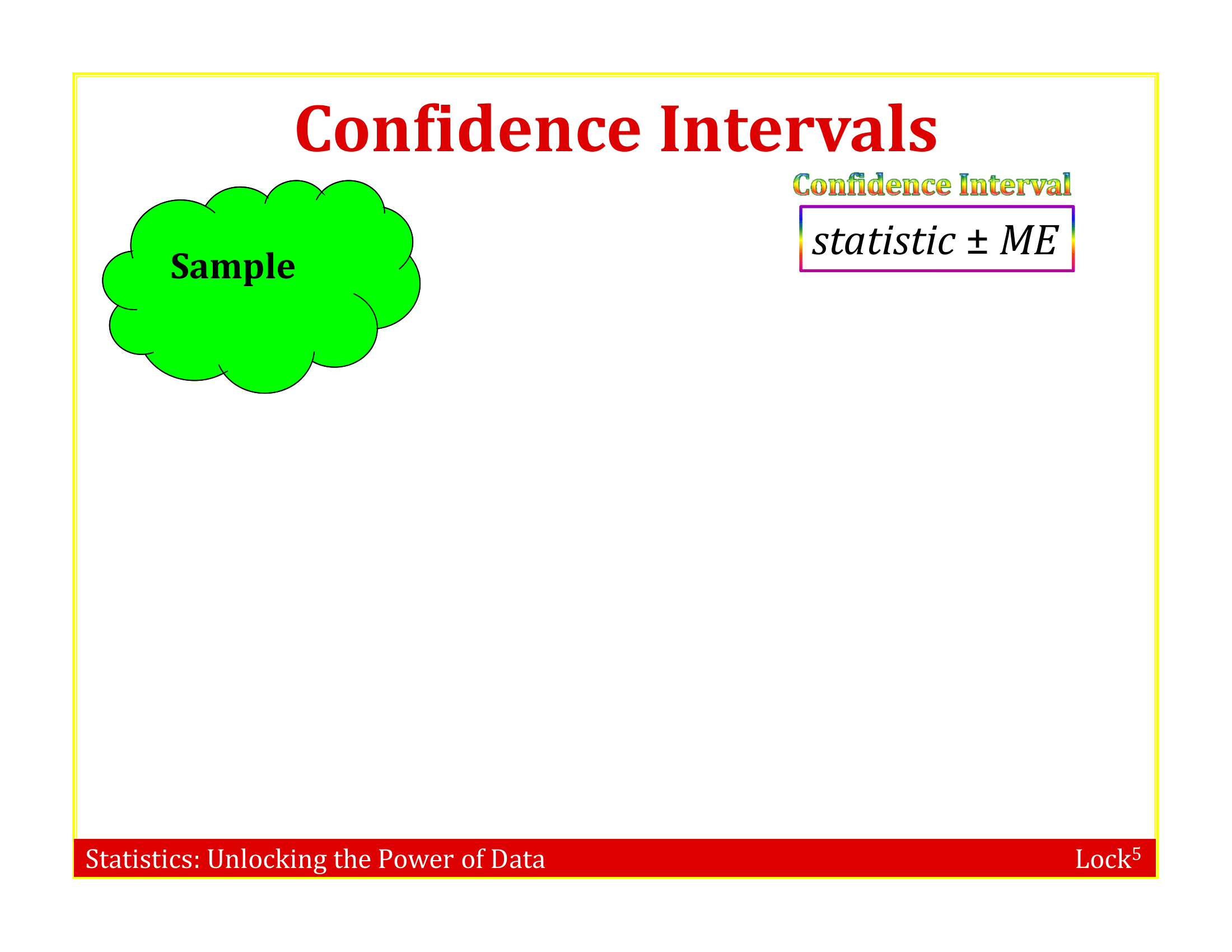
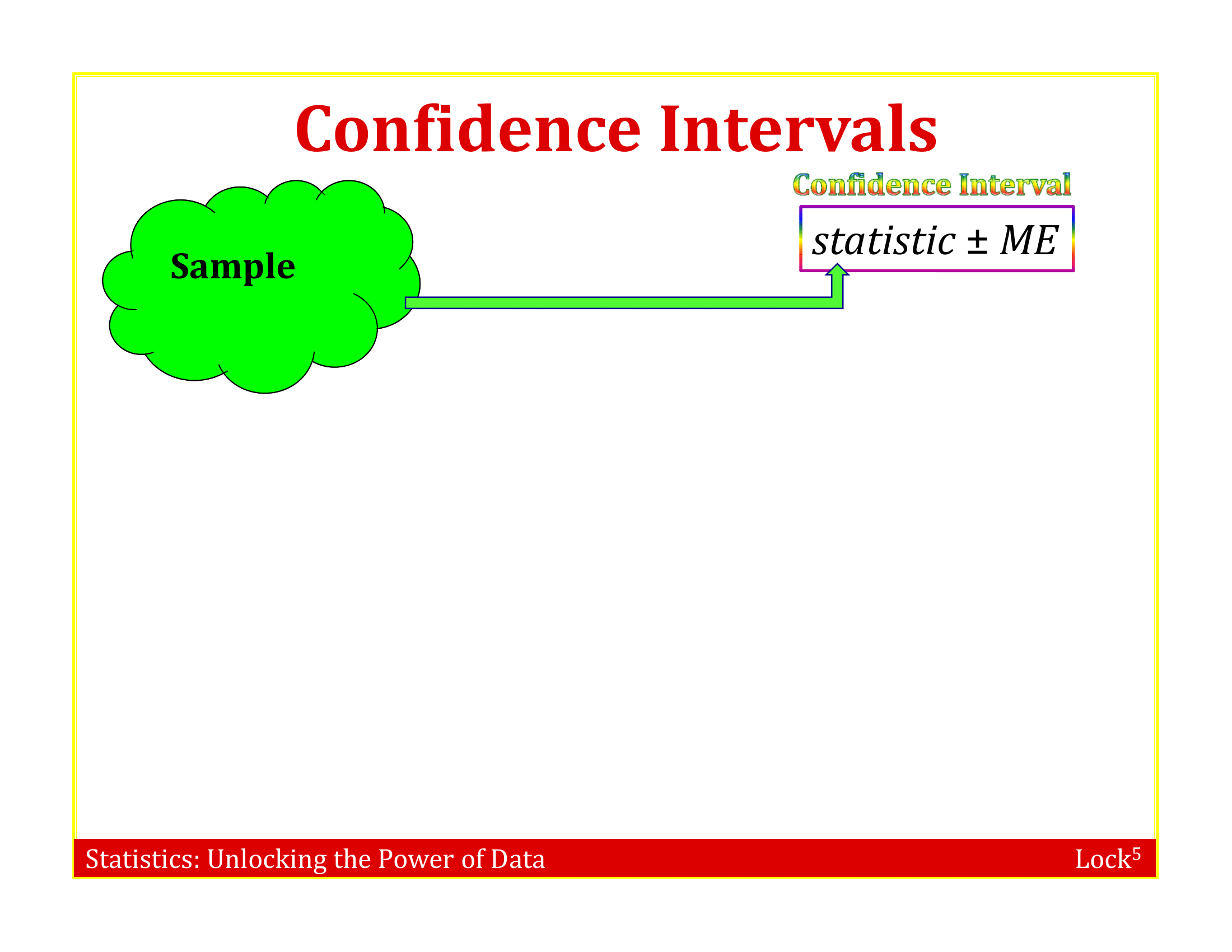
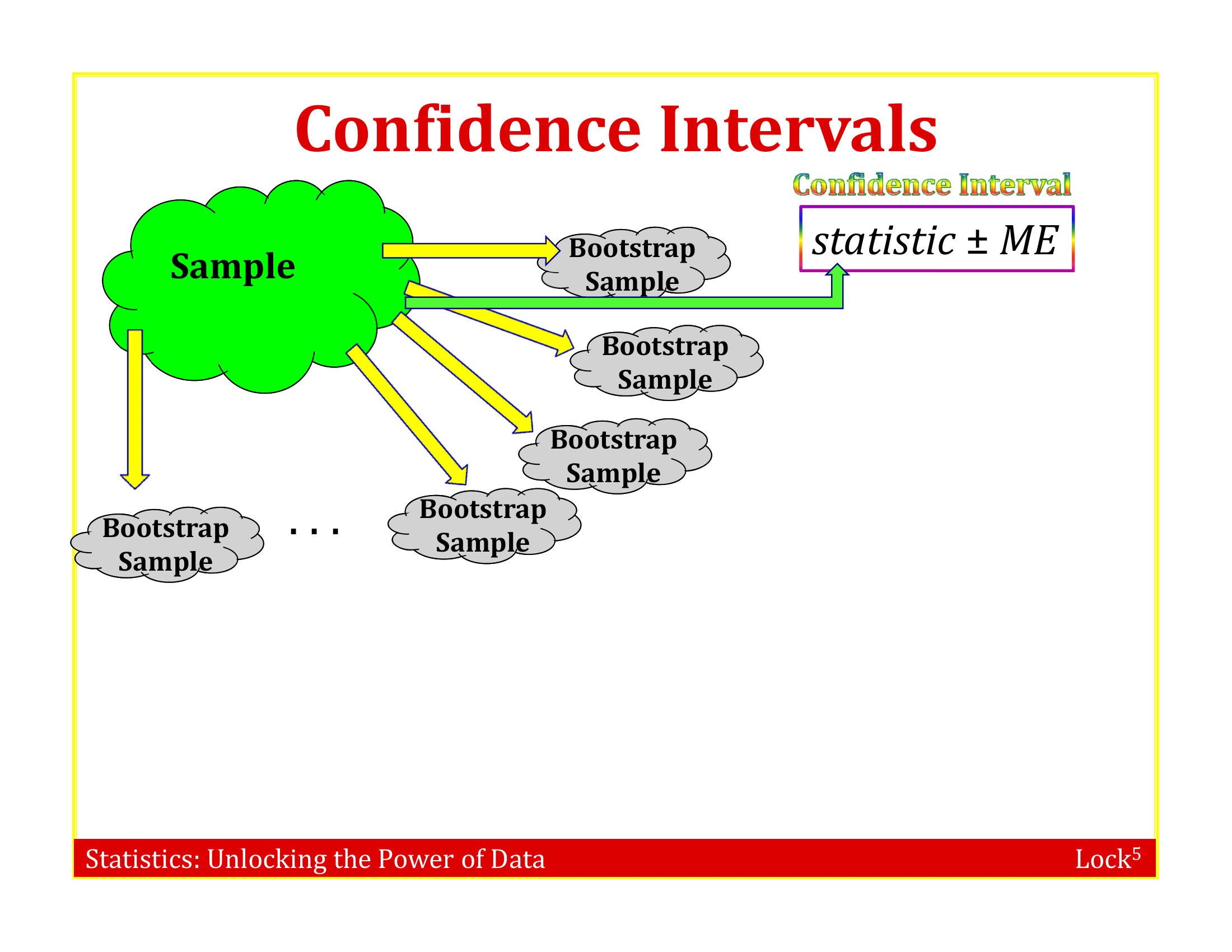
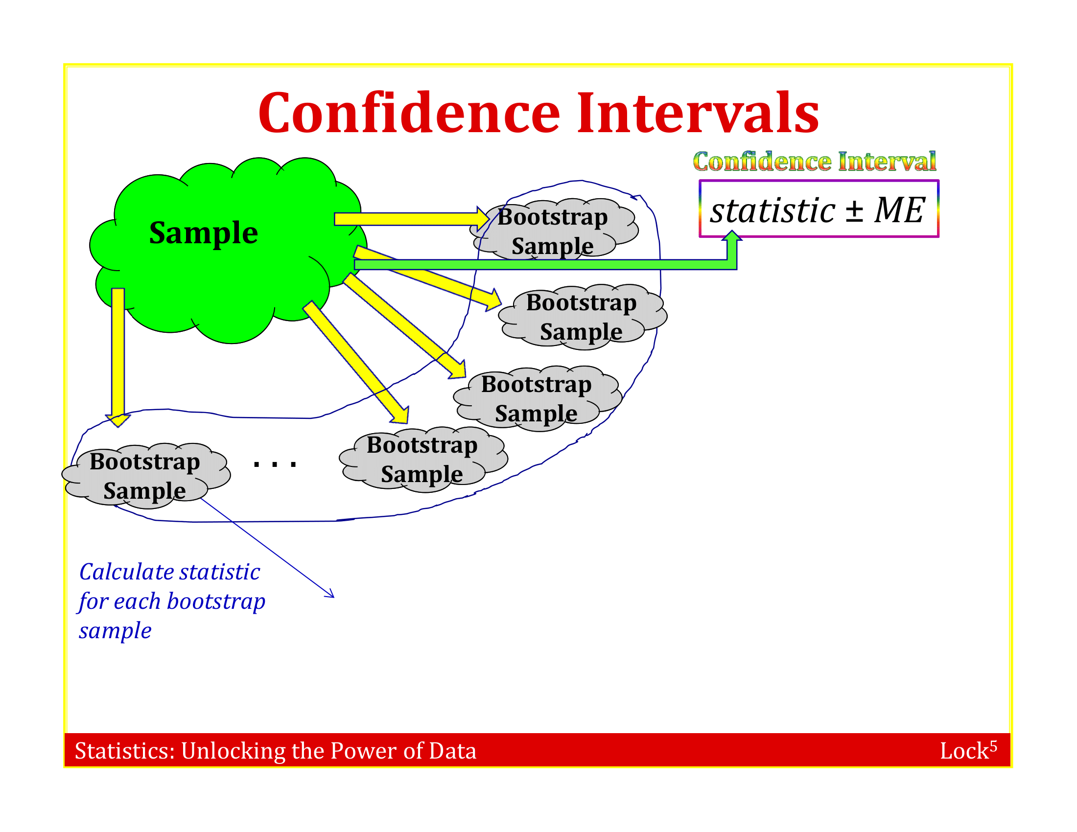
Suppose we have a random sample of 6 people:

Picture of 6 stick figures

Slides demonstrating bootstrapping by resampling 6 stick figures

Slides demonstrating bootstrapping by resampling 6 stick figures

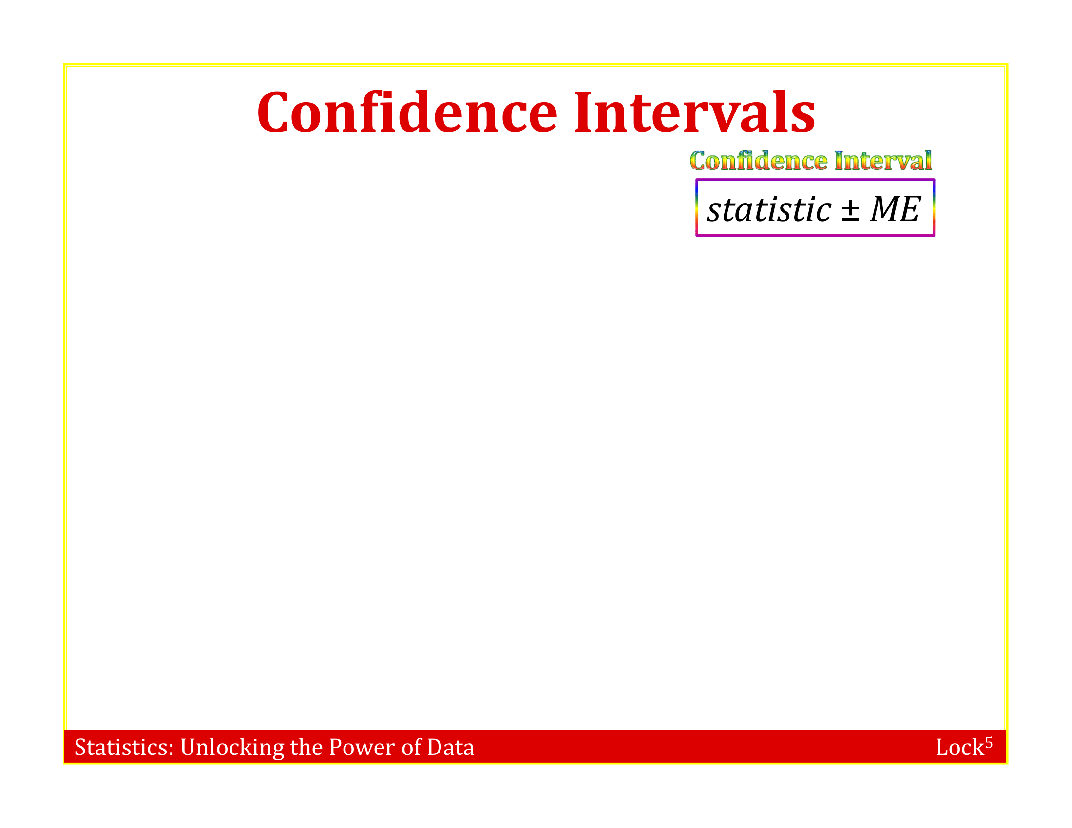
Sampling with Replacement

  • To simulate a sampling distribution, we can just take repeated random samples from this “population” made up of many copies of the sample

  • In practice, we can’t actually make infinite copies of the sample . . .

  • . . . but we can do this by sampling with replacement from the sample we have (each unit can be selected more than once)
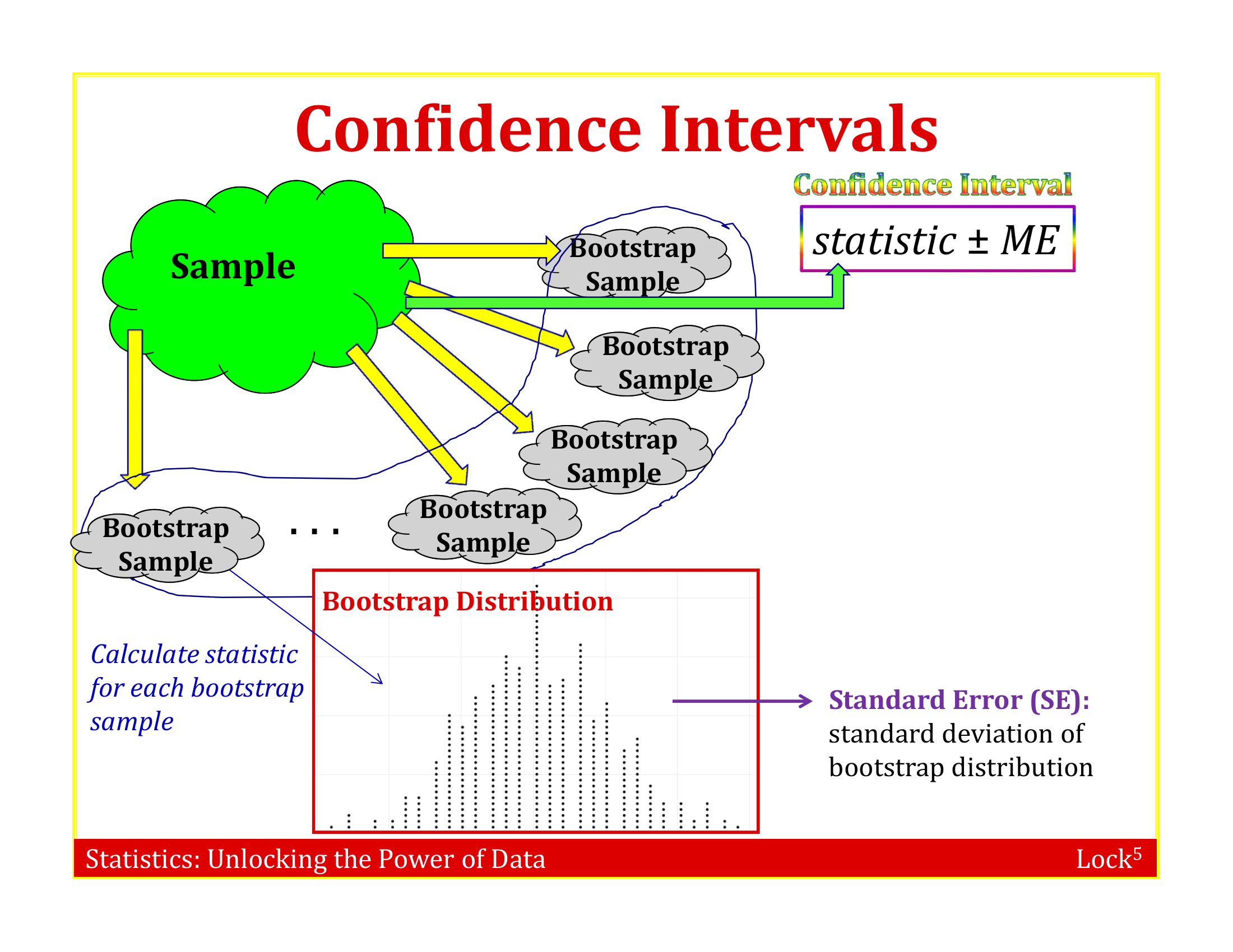
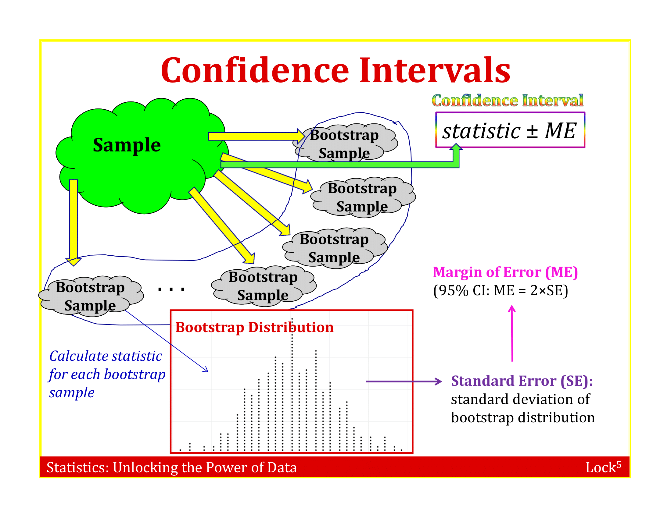
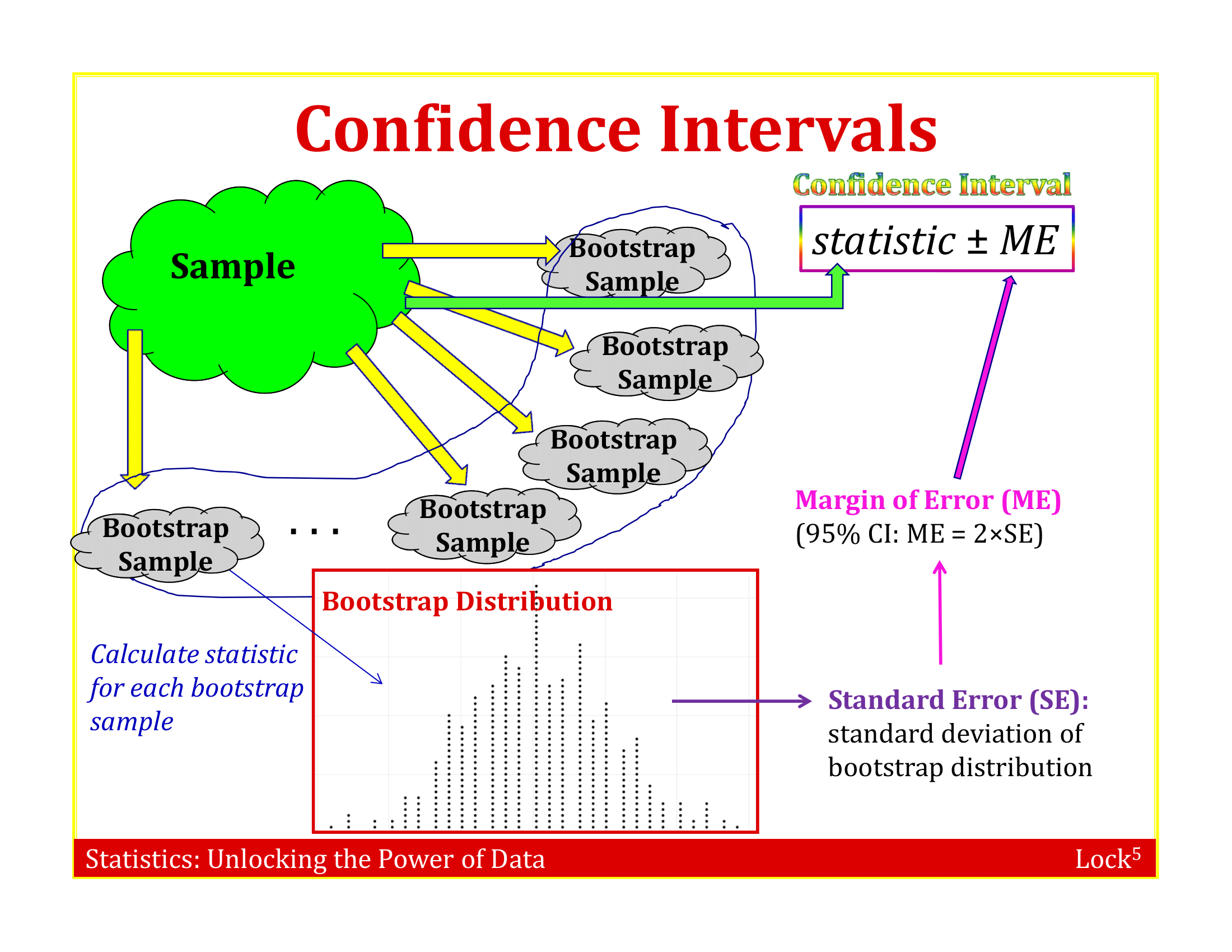
Slides demonstrating bootstrapping by resampling 6 stick figures

Slides demonstrating bootstrapping by resampling 6 stick figures

Slides demonstrating bootstrapping by resampling 6 stick figures

Slides demonstrating bootstrapping by resampling 6 stick figures

Slides demonstrating bootstrapping by resampling 6 stick figures

Slides demonstrating bootstrapping by resampling 6 stick figures

Slides demonstrating bootstrapping by resampling 6 stick figures

Slides demonstrating bootstrapping by resampling 6 stick figures

Bootstrap Sample

Your original sample has data values

18, 19, 19, 20, 21

Is the following a possible bootstrap sample: 18, 19, 20, 21, 22

No, 22 is not a value from the original sample

Is the following a possible bootstrap sample: 18, 19, 20, 21

NO, Bootstrap samples must be the same size as the original sample

Is the following a possible bootstrap sample: 18, 18, 19, 20, 21

YES. Same size, could be gotten by sampling with replacement

Bootstrap

  • A bootstrap sample is a random sample taken with replacement from the original sample, of the same size as the original sample

  • A bootstrap statistic is the statistic computed on a bootstrap sample

  • A bootstrap distribution is the distribution of many bootstrap statistics

Illustration of a bootstrap distribution

Illustration of a bootstrap distribution

Illustration of a bootstrap distribution

Illustration of a bootstrap distribution

Illustration of a bootstrap distribution

Illustration of a bootstrap distribution

Illustration of a bootstrap distribution

Illustration of a bootstrap distribution

Illustration of a bootstrap distribution

Why “Bootstrap”?

“Pull yourself up by your bootstraps”

  • Lift yourself in the air simply by pulling up on the laces of your boots

  • Metaphor for accomplishing an “impossible” task without any outside help

Bootstrap versus Sampling Distribution

  • The sampling distribution should be centered on the population parameter
  • The bootstrap distribution should be centered on the sample statistic

  • Luckily, we don’t care about the center . . . we care about the variability!

Bootstrap versus Sampling Distribution

  • The variability of the bootstrap statistics should be similar to the variability of the sample statistics
  • The standard error of a statistic can be estimated using the standard deviation of the bootstrap distribution!

Mimic Original Sampling Design

What do we do if we have clustered data (multiple obs. on same sampling unit)?

  • Sample clusters with replacement (keeping all observations associated with the cluster)
  • Number of clusters in the bootstrap sample is the same as in the original sample
  • Treats “clusters” as independent

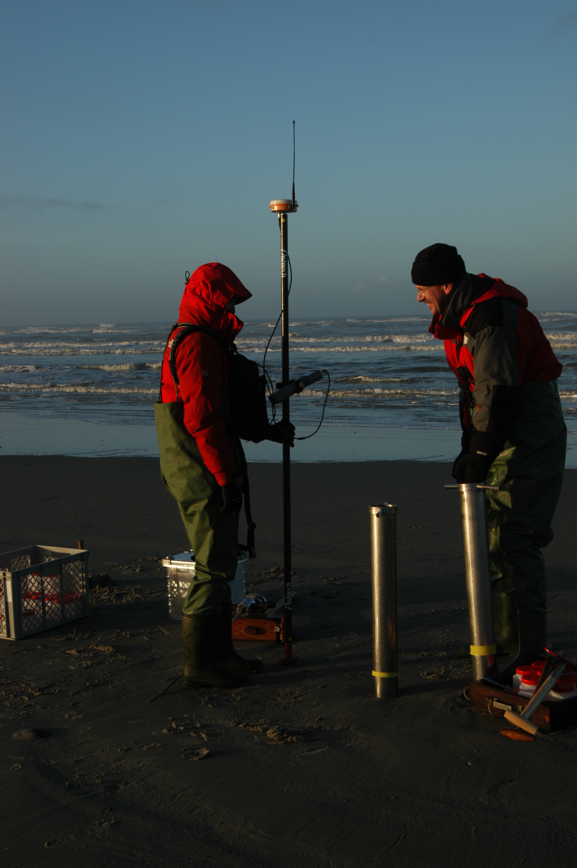
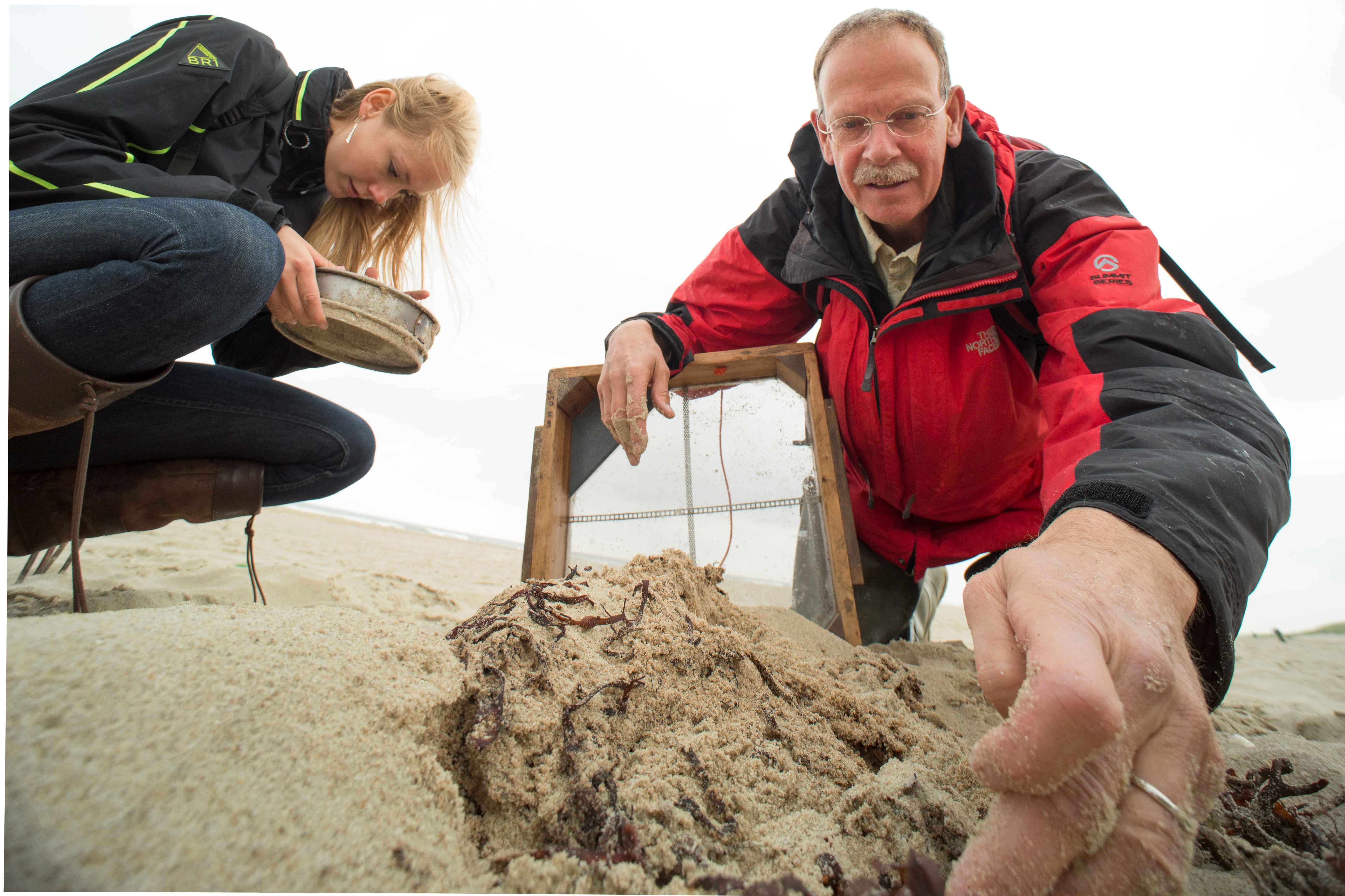
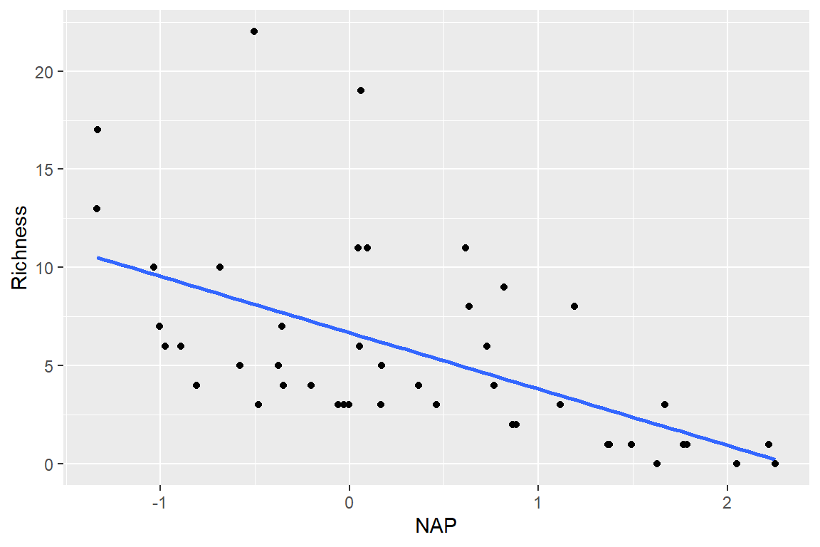
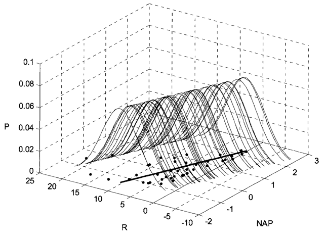
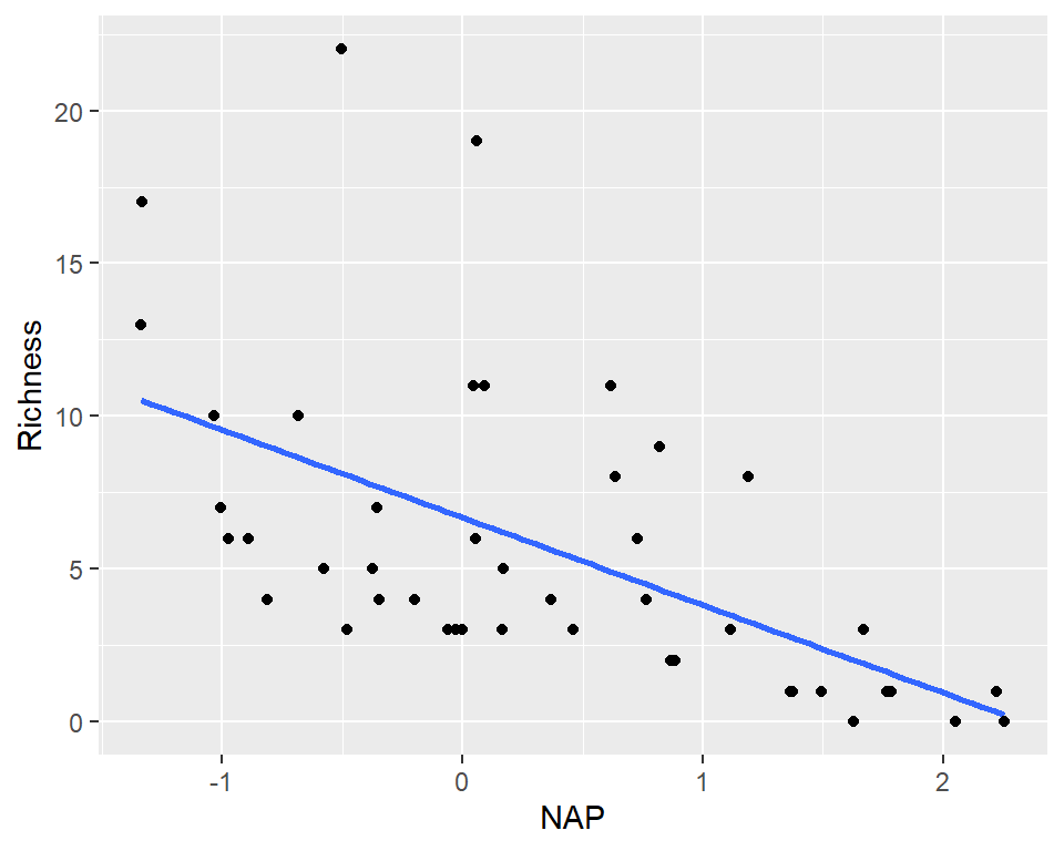
RIKZ Data - Bootstrapping

Cluster-level bootstrapping

Example of a cluster level bootstrap resampling clusters with replacement

Cluster-level bootstrap

This approach is most appropriate when:

  • clusters have equal numbers of observations (all have 5 in this case)
  • our interest lies in predictors that do not vary within a cluster

Example

The code below shows how you can get 1 bootstrap data set using cluster resampling:

# let's use the bootstrap to deal with non-constant variance and clustering
   uid<-unique(RIKZdat$Beach)
   nBeach<-length(uid)

# Single bootstrap sample & fit
  (bootids<-data.frame(Beach=sample(uid, nBeach, replace=T)))
  Beach
1     9
2     1
3     6
4     7
5     6
6     5
7     3
8     6
9     3
  bootdat<-merge(bootids, RIKZdat)  
  table(bootdat$Beach)

 1  3  5  6  7  9 
 5 10  5 15  5  5 

Summary

  • To understand how a bootstrap can be used to quantify uncertainty, particularly when assumptions of linear regression may not be met.

  • To further your coding skills by implementing a cluster-level bootstrap appropriate for certain types of data sets containing repeated observations.