Multiple Regression

FW8051 Statistics for Ecologists

Learning Goals

1. Understand regression analysis with matrix notation.
2. Become familiar with creating dummy variables for categorical regressors
3. Interpret the results of regression analyses with categorical and quantitative variables

Matrix Notation for Regression

Recall: \(Y_i = \beta_0 + \beta_1X_i + \epsilon_i \quad (i = 1, \ldots, n)\)

• This implies:

\[\begin{eqnarray*} Y_1 & = & \beta_0 + \beta_1X_1 + \epsilon_1 \\ Y_2 & = & \beta_0 + \beta_1X_2 + \epsilon_2 \\ & \vdots & \\ Y_n & = & \beta_0 + \beta_1X_n + \epsilon_n \end{eqnarray*}\]

• We can extract this set of equations with matrices.

Matrix Notation for Regression

\[\begin{eqnarray*} Y_1 & = & \beta_0 + \beta_1X_1 + \epsilon_1 \\ Y_2 & = & \beta_0 + \beta_1X_2 + \epsilon_2 \\ & \vdots & \\ Y_n & = & \beta_0 + \beta_1X_n + \epsilon_n \end{eqnarray*}\]

\[\begin{equation*} Y_{n\times1} = \begin{bmatrix}Y_1 \\ Y_2 \\ \vdots \\ Y_n \end{bmatrix} X_{n\times2} = \begin{bmatrix} 1 & X_1 \\ 1 & X_2 \\ \vdots & \vdots \\ 1 & X_n \end{bmatrix} \beta_{2\times1} = \begin{bmatrix} \beta_0 \\ \beta_1 \end{bmatrix} \epsilon_{n\times1} = \begin{bmatrix} \epsilon_1 \\ \epsilon_2 \\ \vdots \\ \epsilon_n \end{bmatrix} \end{equation*}\]

Matrix Notation for Regression

\[\begin{eqnarray*} Y_1 & = & \beta_0 + \beta_1X_1 + \epsilon_1 \\ Y_2 & = & \beta_0 + \beta_1X_2 + \epsilon_2 \\ & \vdots & \\ Y_n & = & \beta_0 + \beta_1X_n + \epsilon_n \end{eqnarray*}\]

\[\begin{equation*} \begin{bmatrix}Y_1 \\ Y_2 \\ \vdots \\ Y_n \end{bmatrix} = \begin{bmatrix}1 & X_1 \\ 1 & X_2 \\ \vdots & \vdots \\ 1 & X_n \end{bmatrix} \times \begin{bmatrix} \beta_0 \\ \beta_1 \end{bmatrix} + \begin{bmatrix} \epsilon_1 \\ \epsilon_2 \\ \vdots \\ \epsilon_n \end{bmatrix} \end{equation*}\]

Matrix Notation for Regression

Also, recall that \(\epsilon \sim \text{N}(0, \sigma^2)\).

• The assumption of independence can be shown with the variance covariance matrix for \(\epsilon\):

\[\begin{equation*} \sigma^2_{\epsilon_{n\times n}} = \begin{bmatrix} \sigma^2 & 0 & 0 & \cdots & 0\\ 0 & \sigma^2 & 0 & \cdots & 0 \\ 0 & 0 & \sigma^2 & \cdots & 0 \\ \vdots & \vdots & \vdots & \ddots & \vdots \\ 0 & 0 & 0 & \cdots & \sigma^2 \end{bmatrix} \end{equation*}\]

• The \((i,i)\) entry = var\((y_i)\)
• The \((i,j)\) entry = cov\((y_i, y_j)\)

Matrix Notation for Regression

Think-Pair-Share

Simple linear regression (i.e., 1 regressor):

\[\begin{equation*} \begin{bmatrix}Y_1 \\ Y_2 \\ \vdots \\ Y_n \end{bmatrix} = \begin{bmatrix}1 & X_1 \\ 1 & X_2 \\ \vdots & \vdots \\ 1 & X_n \end{bmatrix} \times \begin{bmatrix} \beta_0 \\ \beta_1 \end{bmatrix} + \begin{bmatrix} \epsilon_1 \\ \epsilon_2 \\ \vdots \\ \epsilon_n \end{bmatrix} \end{equation*}\]

If we have two regressors (i.e., multiple linear regression), what would the \(X\) and \(\beta\) matrices look like?

Matrix Notation for Regression

We can generalize this matrix notation for any number (\(p-1\)) of regressors: \[\begin{equation*} Y_{[n\times1]} = X_{[n\times p]}\beta_{[p\times 1]} + \epsilon_{[n\times 1]} \end{equation*}\]

\[\begin{equation*} \begin{bmatrix}Y_1 \\ Y_2 \\ \vdots \\ Y_n \end{bmatrix} = \begin{bmatrix}1 & X_{11} & X_{12} & \cdots & X_{1,p-1} \\ 1 & X_{21} & X_{22} & \cdots & X_{2,p-1} \\ \vdots & \vdots & \vdots & & \vdots \\ 1 & X_{n1} & X_{n2} & \cdots & X_{n,p-1} \end{bmatrix} \times \begin{bmatrix} \beta_0 \\ \beta_1 \\ \vdots \\ \beta_{p-1} \end{bmatrix} + \begin{bmatrix} \epsilon_1 \\ \epsilon_2 \\ \vdots \\ \epsilon_n \end{bmatrix} \end{equation*}\]

Note, I am using 2 subscripts (the first indexes each observation; the second indexes each variable in the model).

Multiple linear regression

With multiple (\(p-1\)) explanatory variables, the multiple linear regression model is:

\[Y_i = \beta_0 + \beta_1X_{i1} + \beta_2X_{i2} + \cdots + \beta_{p-1}X_{i,p-1} + \epsilon_i\] \[\epsilon \sim \text{N}(0, \sigma^2)\]

Or, \[Y_i \sim \text{N}(\mu_i, \sigma^2)\] \[\mu_i = \beta_0 + \beta_1X_{i1} + \cdots + \beta_{p-1}X_{i,p-1}\]

We can use lm to find estimates of intercept (\(\beta_0\)) and slope parameters (\(\beta_1, \beta_2, \ldots\)) that minimize SSE:

\(SSE =\sum_i^n(Y_i-\hat{Y}_i)^2 = \sum_i^n(Y_i-[\beta_0 + \beta_1X_{1,i} + \ldots+\beta_{p-1}X_{i,p-1}])^2\)

Multiple Linear Regression

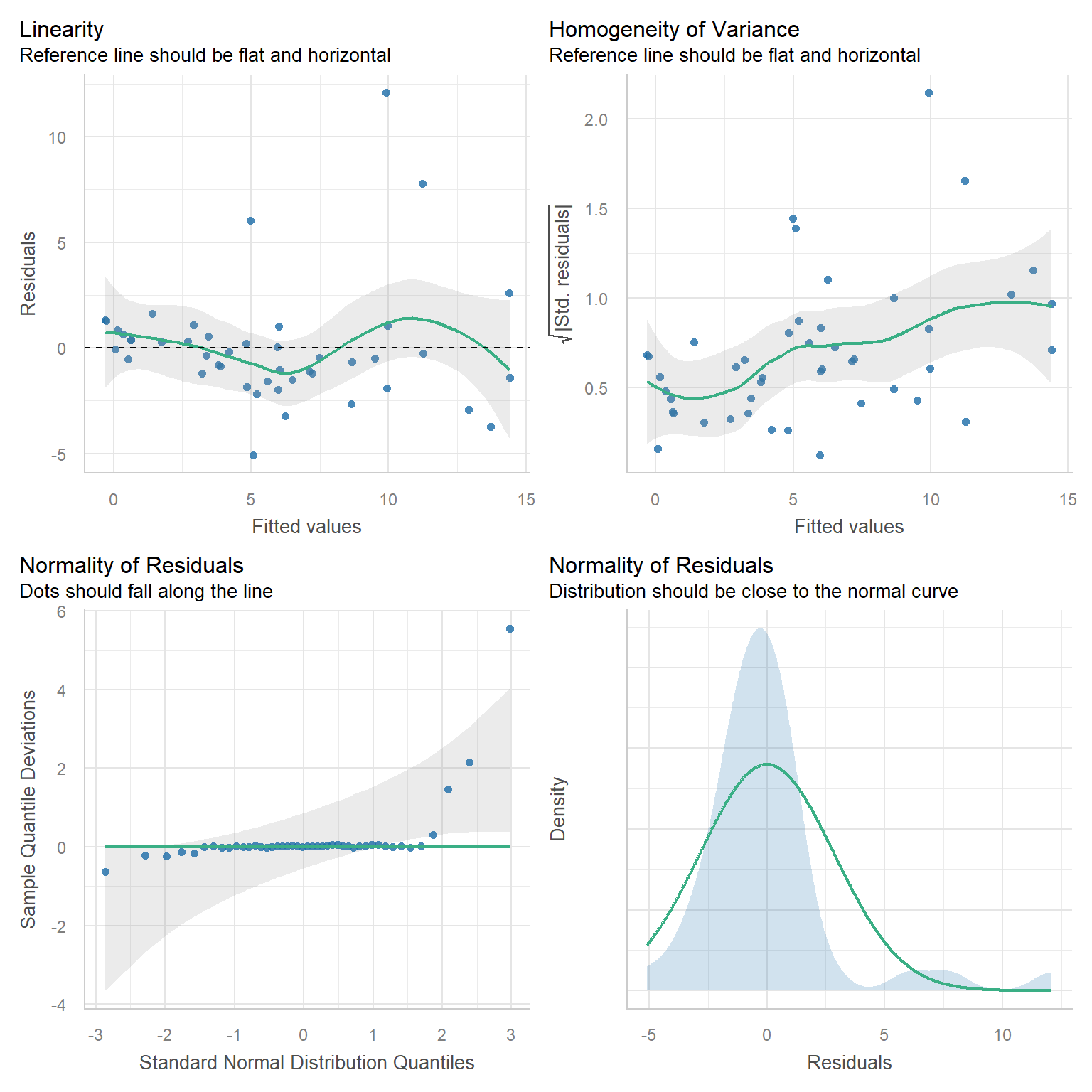
We have the same assumptions (HILE Gauss) and can use the same diagnostic plots.

However, it’s important to diagnose the degree to which explanatory variables are correlated with each other (will address in more detail when we cover multicollinearity).

The Coefficient of Determination (R\(^2= SSR/SST\)) is calculated the same way, with:

• \(SST_{df=n-1} = \sum_i^n(Y_i-\bar{Y})^2\)
  
• \(SSE_{df=n-p} = \sum_i^n(Y_i-\hat{Y})^2\)
  
• \(SSR_{df=p-1} = SST-SSE = \sum_i^n(\hat{Y}_i-\bar{Y})^2\)

In section 8, we will discuss an adjusted R\(^2\) which is more useful when comparing models.

Mutliple Predictors and RIKZ data

• Assuming, naively, that observations are independent, we already established the relationship between Richness (\(\mathrm{R}\)) and relative elevation (\(\mathrm{NAP}\)):

\[\begin{equation*} \hat{\mathrm{R}}_i=6.886-2.867\mathrm{NAP}_i \end{equation*}\]

What if we also hypothesized that humus (\(\mathrm{H}\), amount of organic material) would affect Richness NAP?

• The multiple linear regression model would look like: \[\begin{equation*} \hat{\mathrm{R}}_i=\beta_0 + \beta_1\mathrm{NAP}_i + \beta_2\mathrm{H}_i + \epsilon_i \end{equation*}\]

\(R_i = \beta_0 + \beta_1NAP_i + \beta_2H_i + \epsilon_i\)

  lmfit3<-lm(Richness~NAP+humus, data=RIKZdat)
  summary(lmfit3)

Call:
lm(formula = Richness ~ NAP + humus, data = RIKZdat)

Residuals:
   Min     1Q Median     3Q    Max 
-4.767 -2.464 -0.891  1.389 15.277 

Coefficients:
            Estimate Std. Error t value Pr(>|t|)    
(Intercept)   5.4592     0.8304   6.575 5.92e-08 ***
NAP          -2.5123     0.6227  -4.035 0.000226 ***
humus        21.9424     9.7098   2.260 0.029080 *  
---
Signif. codes:  0 '***' 0.001 '**' 0.01 '*' 0.05 '.' 0.1 ' ' 1

Residual standard error: 3.974 on 42 degrees of freedom
Multiple R-squared:  0.3978,    Adjusted R-squared:  0.3691 
F-statistic: 13.87 on 2 and 42 DF,  p-value: 2.372e-05

Model Comparison

We can compare models: \[\begin{eqnarray*} \hat{\mathrm{R}}_i & = & 6.886 - 2.867\mathrm{NAP}_i \\ \hat{\mathrm{R}}_i & = & 5.459 - 2.512\mathrm{NAP}_i + 21.942\mathrm{H}_i \end{eqnarray*}\]

Interpretations:

• \(\beta_0\): the expected level of Richness if Humus and NAP both equal 0.

• \(\beta_1\): the change in expected Richness for every 1 unit increase in NAP while holding Humus constant

• \(\beta_2\): the change in expected Richness for every 1 unit increase in Humus while holding NAP constant.

Best-fit plane

Categorical variables

Mandible lengths in mm:

• 10 male and 10 female golden jackals
• From British Museum (Manly 1991)

males<-c(120, 107, 110, 116, 114, 111, 113, 117, 114, 112)
females<-c(110, 111, 107, 108, 110, 105, 107, 106, 111, 111)

Do males and females have, on average, different mandible lengths?

\[H_0: \mu_m = \mu_f \text{ versus } H_a: \mu_m \neq \mu_f\]

T-test

t.test(males, females, var.equal=T)

    Two Sample t-test

data:  males and females
t = 3.4843, df = 18, p-value = 0.002647
alternative hypothesis: true difference in means is not equal to 0
95 percent confidence interval:
 1.905773 7.694227
sample estimates:
mean of x mean of y 
    113.4     108.6 

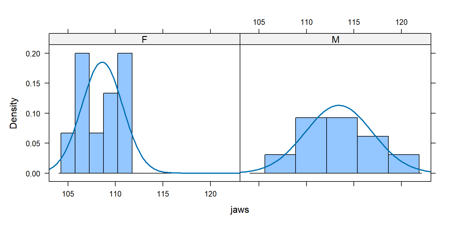
Categorical Variables

We can also test the effect of jackal sex on mandible lengths with a regression model.

• We have to create a data.frame with mandible lengths (quantitative) and sex (categorical)

jawdat <- data.frame(jaws = c(males, females),
                     sex = c(rep("M",10), rep("F", 10)))
head(jawdat) 

  jaws sex
1  120   M
2  107   M
3  110   M
4  116   M
5  114   M
6  111   M

Linear Model

lmfit2<-lm(jaws~sex, data=jawdat)
summary(lmfit2)

Call:
lm(formula = jaws ~ sex, data = jawdat)

Residuals:
   Min     1Q Median     3Q    Max 
  -6.4   -1.8    0.1    2.4    6.6 

Coefficients:
            Estimate Std. Error t value Pr(>|t|)    
(Intercept) 108.6000     0.9741 111.486  < 2e-16 ***
sexM          4.8000     1.3776   3.484  0.00265 ** 
---
Signif. codes:  0 '***' 0.001 '**' 0.01 '*' 0.05 '.' 0.1 ' ' 1

Residual standard error: 3.08 on 18 degrees of freedom
Multiple R-squared:  0.4028,    Adjusted R-squared:  0.3696 
F-statistic: 12.14 on 1 and 18 DF,  p-value: 0.002647

Dummy Variables

This is easier to understand if we use the matrix form of the regression model to view our data.

   jaws sex
16  105   F
18  106   F
2   107   M
13  107   F
17  107   F
14  108   F

\[\begin{equation*} \begin{bmatrix}105 \\ 106 \\ 107 \\ 107 \\ \vdots \end{bmatrix} = \begin{bmatrix}1 & 0 \\ 1 & 0 \\ 1 & 1 \\ 1 & 0 \\ \vdots & \vdots \end{bmatrix} \times \begin{bmatrix} \beta_0 \\ \beta_1 \end{bmatrix} + \begin{bmatrix} \epsilon_1 \\ \epsilon_2 \\ \epsilon_3 \\ \epsilon_4 \\ \vdots \end{bmatrix} \end{equation*}\]

Dummy Variables

• For \(k\) groups of categorical variables, we need to have \(k-1\) dummy variables.
• How many dummy variables do we need for the jackals example?

1 (we have 2 groups)

• Each dummy variable is used as an indicator variable in the model for one group.
  
• In this case, the dummy variable will indicate (i.e., equal 1) for the male jackal observations.

Look at confidence intervals

confint(lmfit2)

                 2.5 %     97.5 %
(Intercept) 106.553472 110.646528
sexM          1.905773   7.694227

t.test(males, females, var.equal=T)

    Two Sample t-test

data:  males and females
t = 3.4843, df = 18, p-value = 0.002647
alternative hypothesis: true difference in means is not equal to 0
95 percent confidence interval:
 1.905773 7.694227
sample estimates:
mean of x mean of y 
    113.4     108.6 

Understanding Model Parameters

Think-Pair-Share

How do we interpret the results?

\[\begin{eqnarray*} Y_i & = & \beta_0 + \beta_1\text{I(sex = male)}_{i} + \epsilon_i\\ & & \text{where }\text{I(sex = male)}_{i}\text{ is 1 if male and 0 if female}\\ \hat{Y}_i & = & 108.6 + 4.8\text{I(sex = male)}_{i} \end{eqnarray*}\]

So, if female :

\(\hat{Y}_i = 108.6 + 4.8(0) = 108.6\)

And if male:

\(\hat{Y}_i = 108.6 + 4.8(1)\)

Note: This parameterization is called “reference” or “effects” coding

Understanding Model Parameters

Alternatively, we can use the “cell-means” or “means” coding:

\[\begin{eqnarray*} Y_i & = & \beta_m\text{I(sex = male)}_{i} + \beta_f\text{I(sex = female)}_{i} + \epsilon_i\\ & & \text{where }\text{I(sex = male)}_{i}\text{ = 1 if male and 0 if female}\\ & & \text{where }\text{I(sex = female)}_{i}\text{ = 1 if female and 0 if male} \end{eqnarray*}\]

In R: lm(jaws~sex-1, data=jawdat)

Reference vs Cell Means Coding

lmfit2b<-lm(jaws~sex, data=jawdat)
summary(lmfit2b)

Call:
lm(formula = jaws ~ sex, data = jawdat)

Residuals:
   Min     1Q Median     3Q    Max 
  -6.4   -1.8    0.1    2.4    6.6 

Coefficients:
            Estimate Std. Error t value Pr(>|t|)    
(Intercept) 108.6000     0.9741 111.486  < 2e-16 ***
sexM          4.8000     1.3776   3.484  0.00265 ** 
---
Signif. codes:  0 '***' 0.001 '**' 0.01 '*' 0.05 '.' 0.1 ' ' 1

Residual standard error: 3.08 on 18 degrees of freedom
Multiple R-squared:  0.4028,    Adjusted R-squared:  0.3696 
F-statistic: 12.14 on 1 and 18 DF,  p-value: 0.002647

lmfit2b<-lm(jaws~sex-1, data=jawdat)
summary(lmfit2b)

Call:
lm(formula = jaws ~ sex - 1, data = jawdat)

Residuals:
   Min     1Q Median     3Q    Max 
  -6.4   -1.8    0.1    2.4    6.6 

Coefficients:
     Estimate Std. Error t value Pr(>|t|)    
sexF 108.6000     0.9741   111.5   <2e-16 ***
sexM 113.4000     0.9741   116.4   <2e-16 ***
---
Signif. codes:  0 '***' 0.001 '**' 0.01 '*' 0.05 '.' 0.1 ' ' 1

Residual standard error: 3.08 on 18 degrees of freedom
Multiple R-squared:  0.9993,    Adjusted R-squared:  0.9992 
F-statistic: 1.299e+04 on 2 and 18 DF,  p-value: < 2.2e-16

Assumptions?

• Equal (constant) variance for the two groups
• Data are normally distributed

library(mosaic)
histogram(~jaws|sex, data=jawdat, cex=1, fit="normal")

Later, we will see how we can relax these assumptions (using either JAGS or gls in the nlme package).

Categorical variables

Recall the RIKZ data.

• Assuming, naively, that observations are independent, we already established the relationship between Richness (\(\mathrm{R}\)) and relative elevation (\(\mathrm{NAP}\)): \[\begin{equation*} \hat{\mathrm{R}}_i=6.886-2.867\mathrm{NAP}_i+\epsilon_i \end{equation*}\]

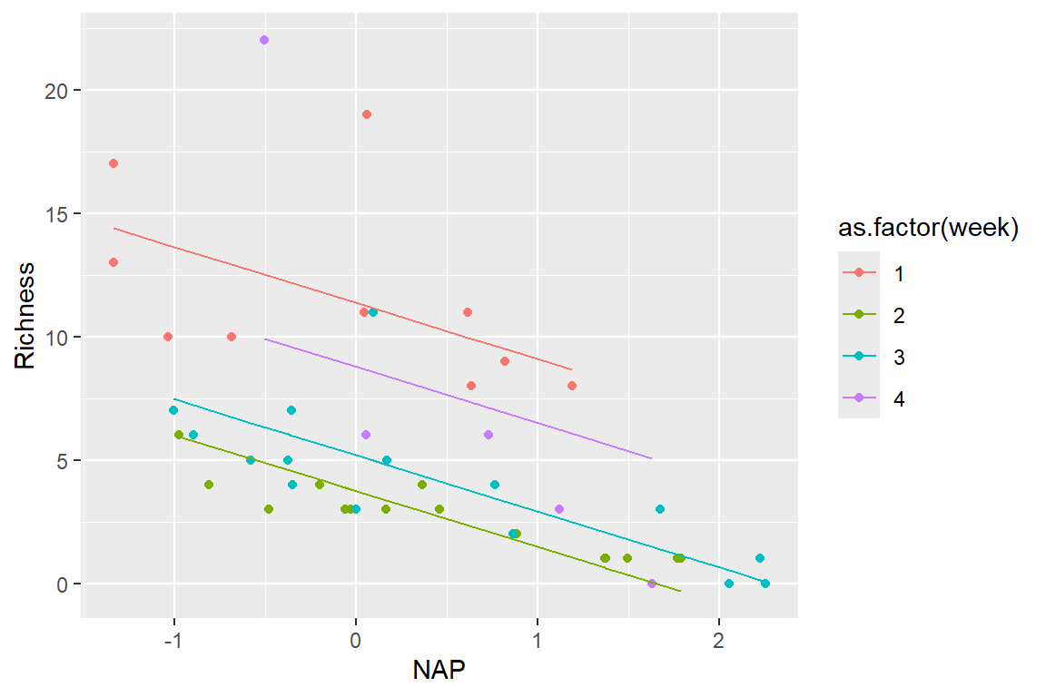
Now, what if we also suspected that the Week the data were collected might affect Richness in addition to NAP?

• Week could be considered continuous, but probably better to analyze it as a nominal variable with 4 categories.
• How many dummy variables will we need to have in order to analyze the effect of Week?

3 (we have 4 groups)

In R, use as.factor(week) to convert to a nominal variable.

Analysis of Covariance Model

lmfit4<-lm(Richness~NAP+as.factor(week), data=RIKZdat)
summary(lmfit4)

Call:
lm(formula = Richness ~ NAP + as.factor(week), data = RIKZdat)

Residuals:
    Min      1Q  Median      3Q     Max 
-5.0788 -1.4014 -0.3633  0.6500 12.0845 

Coefficients:
                 Estimate Std. Error t value Pr(>|t|)    
(Intercept)       11.3677     0.9459  12.017 7.48e-15 ***
NAP               -2.2708     0.4678  -4.854 1.88e-05 ***
as.factor(week)2  -7.6251     1.2491  -6.105 3.37e-07 ***
as.factor(week)3  -6.1780     1.2453  -4.961 1.34e-05 ***
as.factor(week)4  -2.5943     1.6694  -1.554    0.128    
---
Signif. codes:  0 '***' 0.001 '**' 0.01 '*' 0.05 '.' 0.1 ' ' 1

Residual standard error: 2.987 on 40 degrees of freedom
Multiple R-squared:  0.6759,    Adjusted R-squared:  0.6435 
F-statistic: 20.86 on 4 and 40 DF,  p-value: 2.369e-09

Dummy Variables

\[\begin{equation*} Y_i = \beta_0 + \beta_1X_{NAP,i} + \beta_2X_{W2,i} + \beta_3X_{W3,i} + \beta_4X_{W4,i} + \epsilon_i \end{equation*}\]

• where \(X_{W2,i}\), \(X_{W3,i}\), and \(X_{W4,i}\) are indicator variables for Week 2, 3, and 4, respectively.

In matrix form, the data with dummy variables would look like this (try to identify which weeks each observation comes from!):

\[\begin{equation*} \begin{bmatrix}11 \\ 10 \\ 13 \\ 11 \\ \vdots \end{bmatrix} = \begin{bmatrix}1 & 0.045 & 0 & 0 & 1 \\ 1 & -1.036 & 0 & 1 & 0 \\ 1 & -1.336 & 0 & 1 & 0 \\ 1 & 0.616 & 1 & 0 & 0 \\ \vdots & \vdots & \vdots & \vdots & \vdots \end{bmatrix} \times \begin{bmatrix} \beta_0 \\ \beta_1 \\ \beta_2 \\ \beta_3 \\ \beta_4 \end{bmatrix} + \begin{bmatrix} \epsilon_1 \\ \epsilon_2 \\ \epsilon_3 \\ \epsilon_4 \\ \vdots \end{bmatrix} \end{equation*}\]

Use model.matrix in R to see full dataset

Analysis of Covariance (ANCOVA model)

The model is: \[\begin{equation*} Y_i = \beta_0 + \beta_1X_{NAP,i} + \beta_2X_{W2,i} + \beta_3X_{W3,i} + \beta_4X_{W4,i} + \epsilon_i \end{equation*}\]

There is one slope (\(\beta_1\)) relating to the effect of NAP on Richness. In addition, each Week gets its own intercept:

• Week 1: \(Y_i = \beta_0 + \beta_1X_{NAP,i} + \epsilon_i\)

• Week 2: \(Y_i = [\beta_0 + \beta_2(1)] + \beta_1X_{NAP,i} + \epsilon_i\)

• Week 3: \(Y_i = [\beta_0 + \beta_3(1)] + \beta_1X_{NAP,i} + \epsilon_i\)

• Week 4: \(Y_i = [\beta_0 + \beta_4(1)] + \beta_1X_{NAP,i} + \epsilon_i\)

ANCOVA

library(ggplot2)
p <- ggplot(data = cbind(RIKZdat, pred = predict(lmfit4)),
aes(x = NAP, y = Richness, color = as.factor(week)))
p + geom_point() + geom_line(aes(y = pred))

Assumptions

performance::check_model(lmfit4,
    check = c("linearity", "homogeneity", "qq", "normality"))

Means coding

lmfit.ancova.m <- lm(Richness ~ NAP + as.factor(week)-1, data = RIKZdat) 

summary(lmfit.ancova.m)

Call:
lm(formula = Richness ~ NAP + as.factor(week) - 1, data = RIKZdat)

Residuals:
    Min      1Q  Median      3Q     Max 
-5.0788 -1.4014 -0.3633  0.6500 12.0845 

Coefficients:
                 Estimate Std. Error t value Pr(>|t|)    
NAP               -2.2708     0.4678  -4.854 1.88e-05 ***
as.factor(week)1  11.3677     0.9459  12.017 7.48e-15 ***
as.factor(week)2   3.7426     0.8026   4.663 3.44e-05 ***
as.factor(week)3   5.1897     0.7979   6.505 9.24e-08 ***
as.factor(week)4   8.7734     1.3657   6.424 1.20e-07 ***
---
Signif. codes:  0 '***' 0.001 '**' 0.01 '*' 0.05 '.' 0.1 ' ' 1

Residual standard error: 2.987 on 40 degrees of freedom
Multiple R-squared:  0.8604,    Adjusted R-squared:  0.843 
F-statistic: 49.32 on 5 and 40 DF,  p-value: 4.676e-16

Analysis of Covariance (ANCOVA model)

The model is: \[\begin{equation*} Y_i = \beta_1X_{NAP,i} + \beta_2X_{W1,i}+ \beta_3X_{W2,i} + \beta_4X_{W3,i} + \beta_5X_{W4,i} + \epsilon_i \end{equation*}\]

There is one slope (\(\beta_1\)) relating to the effect of NAP on Richness. In addition, each Week gets its own intercept:

• Week 1: \(Y_i = \beta_2 + \beta_1X_{NAP,i} + \epsilon_i\)

• Week 2: \(Y_i = \beta_3 + \beta_1X_{NAP,i} + \epsilon_i\)

• Week 3: \(Y_i = \beta_4 + \beta_1X_{NAP,i} + \epsilon_i\)

• Week 4: \(Y_i = \beta_5 + \beta_1X_{NAP,i} + \epsilon_i\)

Reference vs. Means Coding

lmfit.ancova.r <- lm(Richness ~ NAP + as.factor(week), data = RIKZdat) 

summary(lmfit.ancova.r)

Call:
lm(formula = Richness ~ NAP + as.factor(week), data = RIKZdat)

Residuals:
    Min      1Q  Median      3Q     Max 
-5.0788 -1.4014 -0.3633  0.6500 12.0845 

Coefficients:
                 Estimate Std. Error t value Pr(>|t|)    
(Intercept)       11.3677     0.9459  12.017 7.48e-15 ***
NAP               -2.2708     0.4678  -4.854 1.88e-05 ***
as.factor(week)2  -7.6251     1.2491  -6.105 3.37e-07 ***
as.factor(week)3  -6.1780     1.2453  -4.961 1.34e-05 ***
as.factor(week)4  -2.5943     1.6694  -1.554    0.128    
---
Signif. codes:  0 '***' 0.001 '**' 0.01 '*' 0.05 '.' 0.1 ' ' 1

Residual standard error: 2.987 on 40 degrees of freedom
Multiple R-squared:  0.6759,    Adjusted R-squared:  0.6435 
F-statistic: 20.86 on 4 and 40 DF,  p-value: 2.369e-09

lmfit.ancova.m <- lm(Richness ~ NAP + as.factor(week)-1, data = RIKZdat) 

summary(lmfit.ancova.m)

Call:
lm(formula = Richness ~ NAP + as.factor(week) - 1, data = RIKZdat)

Residuals:
    Min      1Q  Median      3Q     Max 
-5.0788 -1.4014 -0.3633  0.6500 12.0845 

Coefficients:
                 Estimate Std. Error t value Pr(>|t|)    
NAP               -2.2708     0.4678  -4.854 1.88e-05 ***
as.factor(week)1  11.3677     0.9459  12.017 7.48e-15 ***
as.factor(week)2   3.7426     0.8026   4.663 3.44e-05 ***
as.factor(week)3   5.1897     0.7979   6.505 9.24e-08 ***
as.factor(week)4   8.7734     1.3657   6.424 1.20e-07 ***
---
Signif. codes:  0 '***' 0.001 '**' 0.01 '*' 0.05 '.' 0.1 ' ' 1

Residual standard error: 2.987 on 40 degrees of freedom
Multiple R-squared:  0.8604,    Adjusted R-squared:  0.843 
F-statistic: 49.32 on 5 and 40 DF,  p-value: 4.676e-16

Interactions

We should be cautious with interactions:

• In experimental data, interactions should frequently be examined, and often should be examined before testing for main effects.

• In observational studies, data will usually be unbalanced. Interactions should rarely be examined unless though to be important a priori.

Interactions

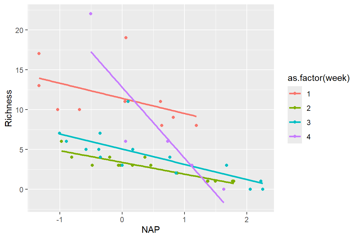
For illustration only, we can naively assume that we think that NAP and Week interact in their effects on Richness.

• Caveat: there’s no real biological reason that week and relative elevation should interact, and the researchers did not design this experiment to test for this interaction.

lmfit.ancovaI <- lm(Richness ~ NAP * as.factor(week), data = RIKZdat)
summary(lmfit.ancovaI)

Call:
lm(formula = Richness ~ NAP * as.factor(week), data = RIKZdat)

Residuals:
    Min      1Q  Median      3Q     Max 
-6.3022 -0.9442 -0.2946  0.3383  7.7103 

Coefficients:
                     Estimate Std. Error t value Pr(>|t|)    
(Intercept)          11.40561    0.77730  14.673  < 2e-16 ***
NAP                  -1.90016    0.87000  -2.184 0.035369 *  
as.factor(week)2     -8.04029    1.05519  -7.620 4.30e-09 ***
as.factor(week)3     -6.37154    1.03168  -6.176 3.63e-07 ***
as.factor(week)4      1.37721    1.60036   0.861 0.395020    
NAP:as.factor(week)2  0.42558    1.12008   0.380 0.706152    
NAP:as.factor(week)3 -0.01344    1.04246  -0.013 0.989782    
NAP:as.factor(week)4 -7.00002    1.68721  -4.149 0.000188 ***
---
Signif. codes:  0 '***' 0.001 '**' 0.01 '*' 0.05 '.' 0.1 ' ' 1

Residual standard error: 2.442 on 37 degrees of freedom
Multiple R-squared:  0.7997,    Adjusted R-squared:  0.7618 
F-statistic: 21.11 on 7 and 37 DF,  p-value: 3.935e-11

Interactions

\(Y_i = \beta_0 + \beta_1X_{NAP,i} +\beta_2X_{W2,i} + \beta_3X_{W3,i} + \beta_4X_{W4,i}+ \beta_5X_{NAP,i}X_{W2,i} + \beta_6X_{NAP,i}X_{W3,i} + \beta_7X_{NAP,i}X_{W4,i} + \epsilon_i\)

There is one slope and one intercept for each week:

• Week 1: \(Y_i = \beta_0 + \beta_1X_{NAP,i} + \epsilon_i\)

• Week 2: \(Y_i = [\beta_0 + \beta_2(1)] + [\beta_1 + \beta_5(1)]X_{NAP,i} + \epsilon_i\)

• Week 3: \(Y_i = [\beta_0 + \beta_3(1)] + [\beta_1 + \beta_6(1)]X_{NAP,i} + \epsilon_i\)

• Week 4: \(Y_i = [\beta_0 + \beta_4(1)] + [\beta_1 + \beta_7(1)]X_{NAP,i} + \epsilon_i\)

Parameters \(\beta_2, \beta_3, \beta_4\) reflect differences in intercepts (from week 1’s intercept).

Parameters \(\beta_5, \beta_6, \beta_7\) reflect differences in slopes (from week 1’s slope).

Interactions

\(Y_i = \beta_0 + \beta_1X_{NAP,i} +\beta_2X_{W2,i} + \beta_3X_{W3,i} + \beta_4X_{W4,i}+ \beta_5X_{NAP,i}X_{W2,i} + \beta_6X_{NAP,i}X_{W3,i} + \beta_7X_{NAP,i}X_{W4,i} + \epsilon_i\)

The data in matrix form (again, try to determine which week each observation comes from!):

\[\begin{equation*} \begin{bmatrix}11 \\ 10 \\ 13 \\ 11 \\ \vdots \end{bmatrix} = \begin{bmatrix}1 & 0.045 & 0 & 0 & 1 & 0 & 0 & 0.045 \\ 1 & -1.036 & 0 & 1 & 0 & 0 & -1.036 & 0\\ 1 & -1.336 & 0 & 1 & 0 & 0 & -1.336 & 0 \\ 1 & 0.616 & 1 & 0 & 0 & 0.616 & 0 & 0 \\ \vdots & \vdots & \vdots & \vdots & \vdots & \vdots & \vdots & \vdots \end{bmatrix} \times \begin{bmatrix} \beta_0 \\ \beta_1 \\ \beta_2 \\ \beta_3 \\ \beta_4 \\ \beta_5 \\ \beta_6 \\ \beta_7 \end{bmatrix} + \begin{bmatrix} \epsilon_1 \\ \epsilon_2 \\ \epsilon_3 \\ \epsilon_4 \\ \vdots \end{bmatrix} \end{equation*}\]

To specify the same model using means coding, we would use:

lmfit.ancovaI.m<-lm(Richness~NAP*as.factor(week)-1-NAP, data=RIKZdat)
summary(lmfit.ancovaI.m)

Call:
lm(formula = Richness ~ NAP * as.factor(week) - 1 - NAP, data = RIKZdat)

Residuals:
    Min      1Q  Median      3Q     Max 
-6.3022 -0.9442 -0.2946  0.3383  7.7103 

Coefficients:
                     Estimate Std. Error t value Pr(>|t|)    
as.factor(week)1      11.4056     0.7773  14.673  < 2e-16 ***
as.factor(week)2       3.3653     0.7136   4.716 3.38e-05 ***
as.factor(week)3       5.0341     0.6784   7.421 7.85e-09 ***
as.factor(week)4      12.7828     1.3989   9.138 5.05e-11 ***
NAP:as.factor(week)1  -1.9002     0.8700  -2.184  0.03537 *  
NAP:as.factor(week)2  -1.4746     0.7055  -2.090  0.04353 *  
NAP:as.factor(week)3  -1.9136     0.5743  -3.332  0.00197 ** 
NAP:as.factor(week)4  -8.9002     1.4456  -6.157 3.85e-07 ***
---
Signif. codes:  0 '***' 0.001 '**' 0.01 '*' 0.05 '.' 0.1 ' ' 1

Residual standard error: 2.442 on 37 degrees of freedom
Multiple R-squared:  0.9138,    Adjusted R-squared:  0.8951 
F-statistic:    49 on 8 and 37 DF,  p-value: < 2.2e-16

In this case, we directly get estimates of the intercepts and slopes for each week.

Interactions

ggplot(RIKZdat, aes(x=NAP, y=Richness, colour=as.factor(week)))+
  geom_smooth(method = "lm", se = FALSE)+geom_point()

Think-Pair-Share

How could we fit a model where the effect of NAP was the same for all weeks except week 4?

lmfit.special <- lm(Richness ~ NAP + as.factor(week) + NAP:I(week==4),
                    data = RIKZdat)
summary(lmfit.special)

Call:
lm(formula = Richness ~ NAP + as.factor(week) + NAP:I(week == 
    4), data = RIKZdat)

Residuals:
    Min      1Q  Median      3Q     Max 
-6.3022 -0.9762 -0.0838  0.6269  7.6894 

Coefficients:
                     Estimate Std. Error t value Pr(>|t|)    
(Intercept)           11.4187     0.7558  15.108  < 2e-16 ***
NAP                   -1.7722     0.3875  -4.573 4.77e-05 ***
as.factor(week)2      -7.9124     0.9996  -7.915 1.23e-09 ***
as.factor(week)3      -6.4463     0.9965  -6.469 1.16e-07 ***
as.factor(week)4       1.3641     1.5623   0.873    0.388    
NAP:I(week == 4)TRUE  -7.1280     1.4652  -4.865 1.92e-05 ***
---
Signif. codes:  0 '***' 0.001 '**' 0.01 '*' 0.05 '.' 0.1 ' ' 1

Residual standard error: 2.387 on 39 degrees of freedom
Multiple R-squared:  0.7983,    Adjusted R-squared:  0.7725 
F-statistic: 30.88 on 5 and 39 DF,  p-value: 1.425e-12

Interactions

Although these results look convincing, remember:

• this an unbalanced design, with only 5 observations during week 4!

table(RIKZdat$week)  

 1  2  3  4 
10 15 15  5 

• Hence, this interaction model should be interpreted with caution unless there was an a priori reason to expect the effect of NAP to vary by week.

Multiple degree of freedom tests

  library(car)
  lm.RIKZ<-lm(Richness~NAP+exposure+as.factor(week), data=RIKZdat)
  Anova(lm.RIKZ)

Anova Table (Type II tests)

Response: Richness
                Sum Sq Df F value    Pr(>F)    
NAP             231.59  1 27.1999 6.335e-06 ***
exposure         24.94  1  2.9289   0.09495 .  
as.factor(week)  73.19  3  2.8654   0.04888 *  
Residuals       332.07 39                      
---
Signif. codes:  0 '***' 0.001 '**' 0.01 '*' 0.05 '.' 0.1 ' ' 1

Multiple df test tests whether all 3 coefficients associated with as.factor(week) are 0 versus the alternative hypothesis that at least 1 is non-zero (all weeks are the same vs. at least one of the weeks differs from the others).

Anova versus anova

• For continuous variables, the p-values from Anova will be identical to the t-test p-values (see exposure variable).

• These tests for (NAP, exposure, week) are conditional on having the other terms included in the model.

• By contrast the anova function which performs “sequential” tests (where, “order of entry” matters!)

  anova(lm(Richness~NAP+exposure+as.factor(week), data=RIKZdat))

Analysis of Variance Table

Response: Richness
                Df Sum Sq Mean Sq F value    Pr(>F)    
NAP              1 357.53  357.53 41.9907 1.117e-07 ***
exposure         1 338.86  338.86 39.7977 1.931e-07 ***
as.factor(week)  3  73.19   24.40  2.8654   0.04888 *  
Residuals       39 332.07    8.51                      
---
Signif. codes:  0 '***' 0.001 '**' 0.01 '*' 0.05 '.' 0.1 ' ' 1

  anova(lm(Richness~as.factor(week)+exposure+NAP, data=RIKZdat))

Analysis of Variance Table

Response: Richness
                Df Sum Sq Mean Sq F value    Pr(>F)    
as.factor(week)  3 534.31 178.104 20.9177 3.060e-08 ***
exposure         1   3.67   3.675  0.4316    0.5151    
NAP              1 231.59 231.593 27.1999 6.335e-06 ***
Residuals       39 332.07   8.514                      
---
Signif. codes:  0 '***' 0.001 '**' 0.01 '*' 0.05 '.' 0.1 ' ' 1

Additional Notes

See section 3.8 in the book for information on how to conduct pairwise comparisons (e.g., we have “4 choose 2” = 6 possible comparisons of different weeks).

See sections 3.12 and 3.13 for information regarding how to test your own hypotheses using contrasts (formed by taking linear combinations of the regression coefficients).

For example, we could test whether the average richness during weeks 1 and 2 differs from the average richness of weeks 3 and 4.

Summary

1. Understand regression analysis with matrix notation.
2. Become familiar with creating dummy variables for categorical regressors
3. Interpret the results of regression analyses with categorical and quantitative variables