So, we can use all the same tools we’ve learned about (e.g., residual plots, t-tests, F-tests, AIC, etc) [note: try writing out the above models in matrix notation!]
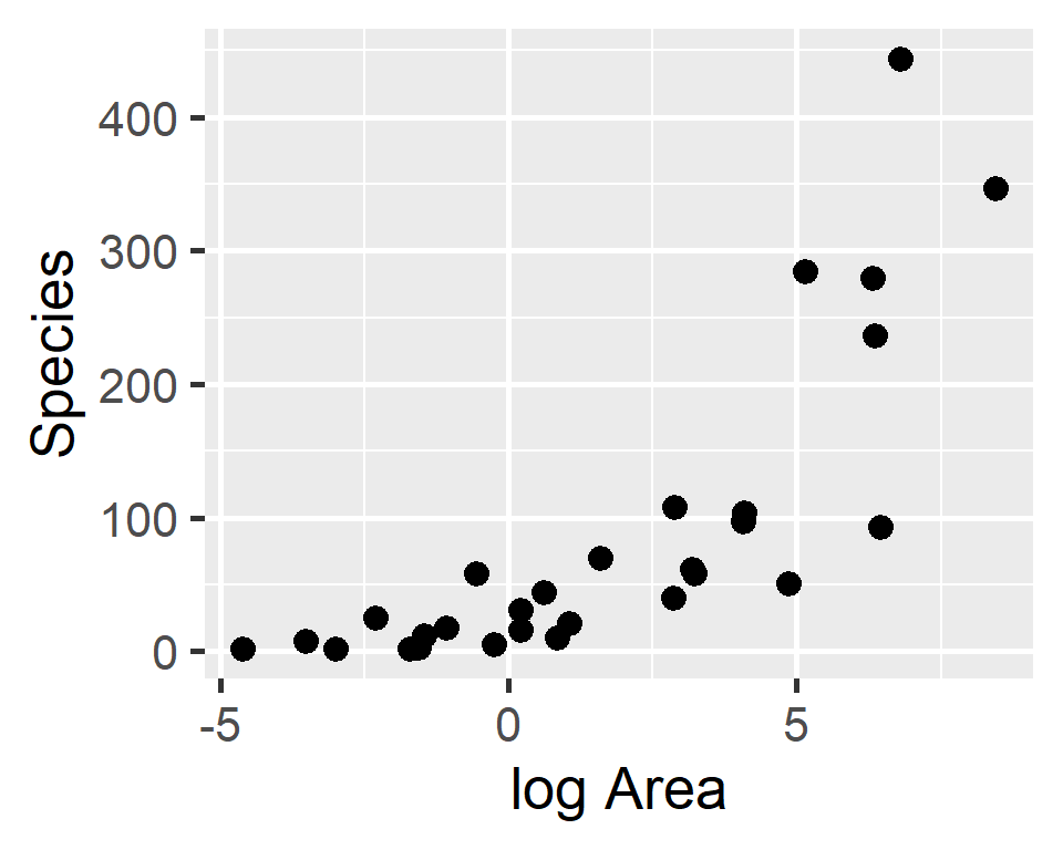
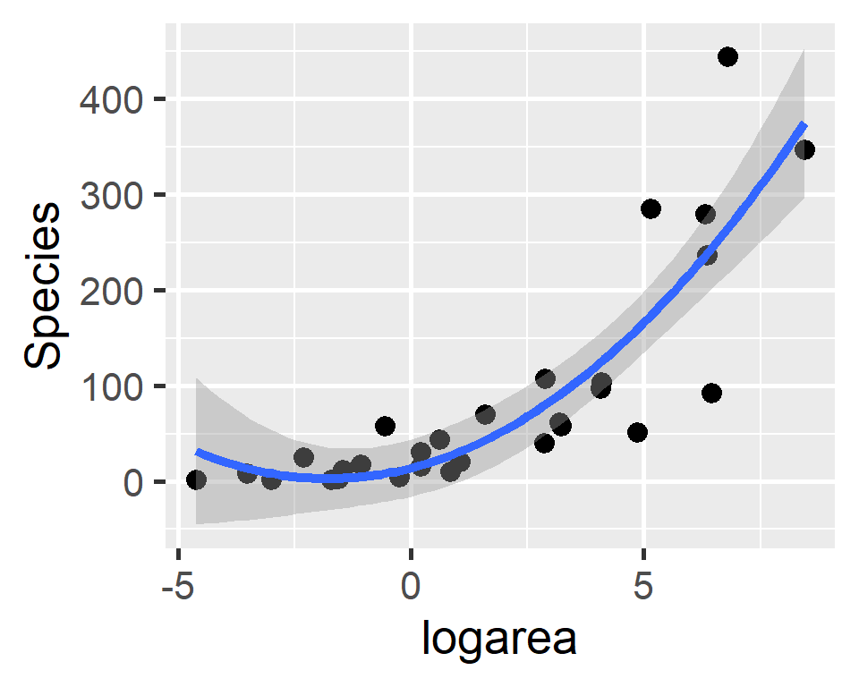
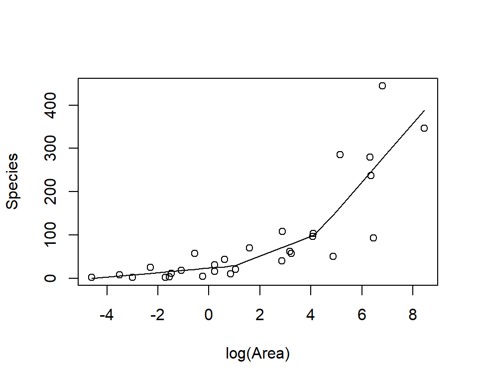
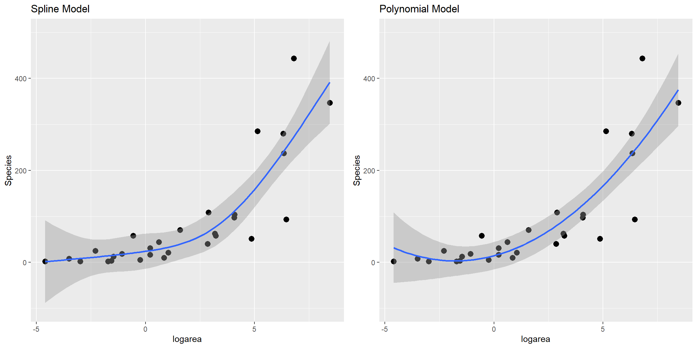
Species-area relationship
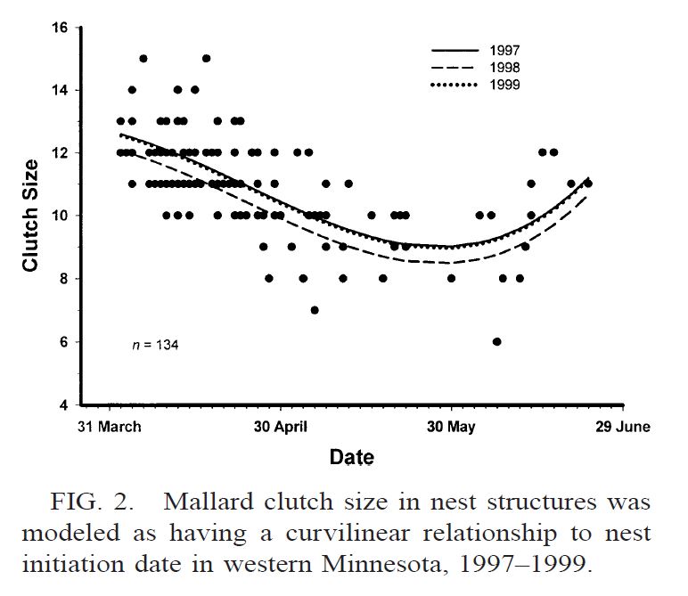
Plant species richness for 29 islands in the Galapagos Islands archipelago (Johnson and Raven 1973)
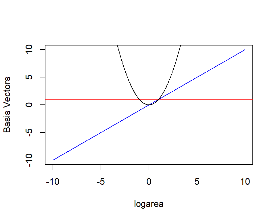
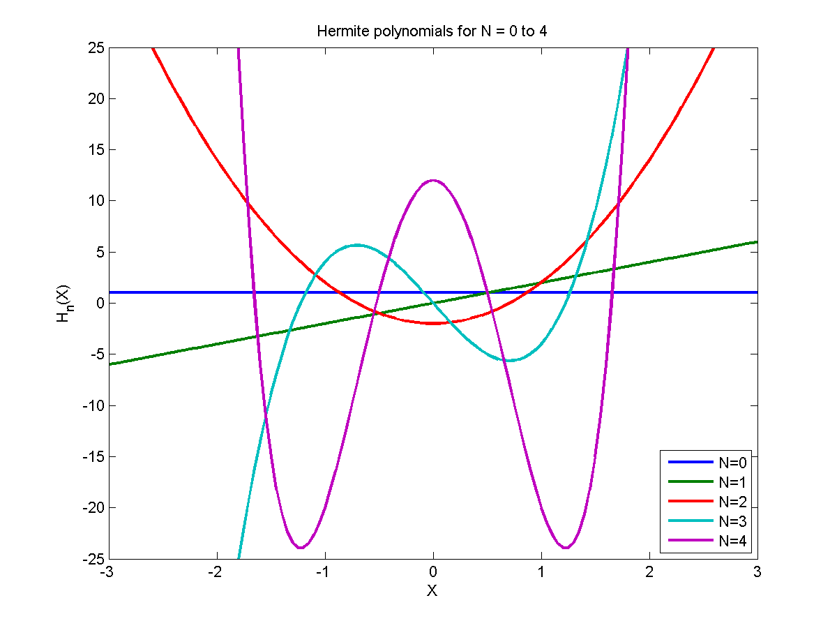
\(E[Y | X]\) is given by a linear combination of a horizontal line (1), a line through the origin (\(X\)), a quadratic centered on the origin (\(X^2\)).
The design matrix for a regression model with \(n\) observations and \(p\) predictors is the matrix with \(n\) rows and \(p\) columns such that the value of the \(j^{th}\) predictor for the \(i^{th}\) observation is located in column \(j\) of row \(i\).
Standard polynomials can cause numerical issues due to differences in scale:
\(X = 100\)\(X^3 = 1,000,000\)
Centering and scaling \(X\) can help.
Alternatively, we can use “orthogonal polynomials” created using poly(raw=FALSE) (the default). See Section 4.10 in the book.
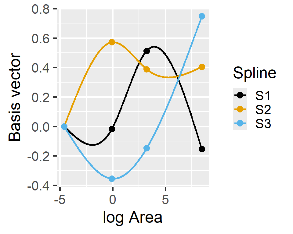
Splines
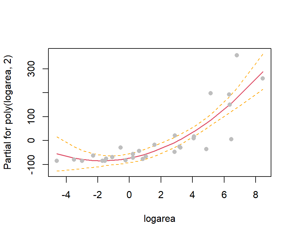
Species-Area relationship
Linear models are often a good approximation over small ranges of \(x\).
Splines
Splines are piecewise polynomials used in curve fitting.
A linear spline is a continuous function formed by connecting linear segments. The points where the segments connect are called the knots of the spline.
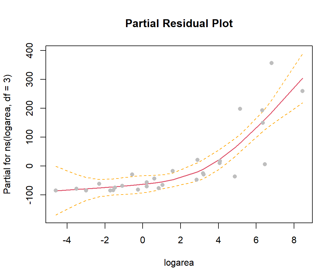
Call:
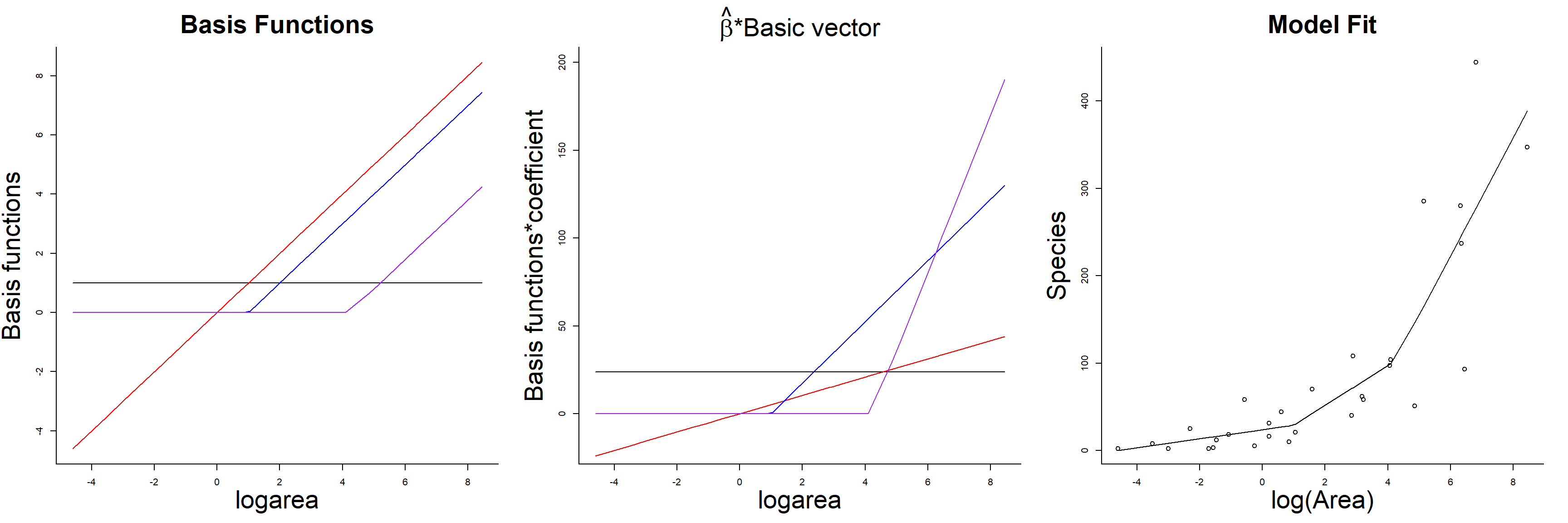
lm(formula = Species ~ logarea + logarea.1 + logarea.4.2, data = gala)
Residuals:
Min 1Q Median 3Q Max
-160.691 -16.547 -4.209 13.133 166.430
Coefficients:
Estimate Std. Error t value Pr(>|t|)
(Intercept) 23.869 17.384 1.373 0.1819
logarea 5.213 8.956 0.582 0.5658
logarea.1 17.464 18.836 0.927 0.3627
logarea.4.2 44.815 23.156 1.935 0.0643 .
---
Signif. codes: 0 '***' 0.001 '**' 0.01 '*' 0.05 '.' 0.1 ' ' 1
Residual standard error: 58.97 on 25 degrees of freedom
Multiple R-squared: 0.7695, Adjusted R-squared: 0.7418
F-statistic: 27.82 on 3 and 25 DF, p-value: 3.934e-08
Basis functions
Left = Basis Functions
Middle = Basis Functions * regression coefficient
Right = Fitted Model
Splines
A spline of degree D is a function formed by connecting polynomial segments of degree D so that:
the function is continuous (no `jumps’)
the function has D-1 continuous derivatives
the D\(^{th}\) derivative is constant between knots
Linear splines (D = 1): first derivative is not constant (can go from increasing to decreasing at a knot)
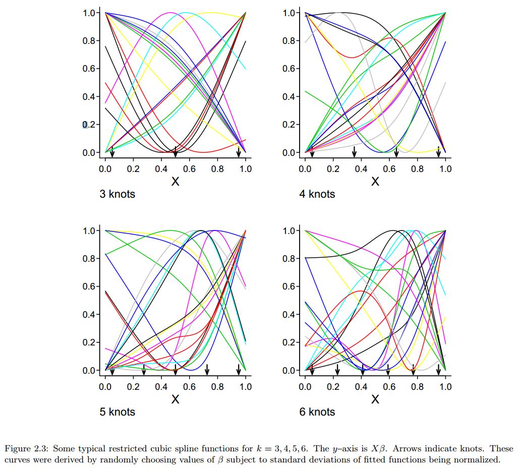
Cubic Regression Splines
Fits a cubic polynomial on segments of the data
D-1 = 2 continuous derivatives everywhere (even at the knot locations)
the first derivative (tells us if the function is increasing or decreasing) is continuous (even at the knots)
the second derivative (tell us about curvature) is constant (even at the knots)
Ensures that the fit is “smooth” at the connections (knot locations)
Truncated Power Basis
The truncated polynomial of degree D associated with a knot \(\xi_k\) is the function which is equal to 0 to the left of \(\xi_k\) and equal to \((x - \xi_k)^D\) to the right of \(\xi_k\).
where \(f(x_1)\) can be modeled in a variety of ways
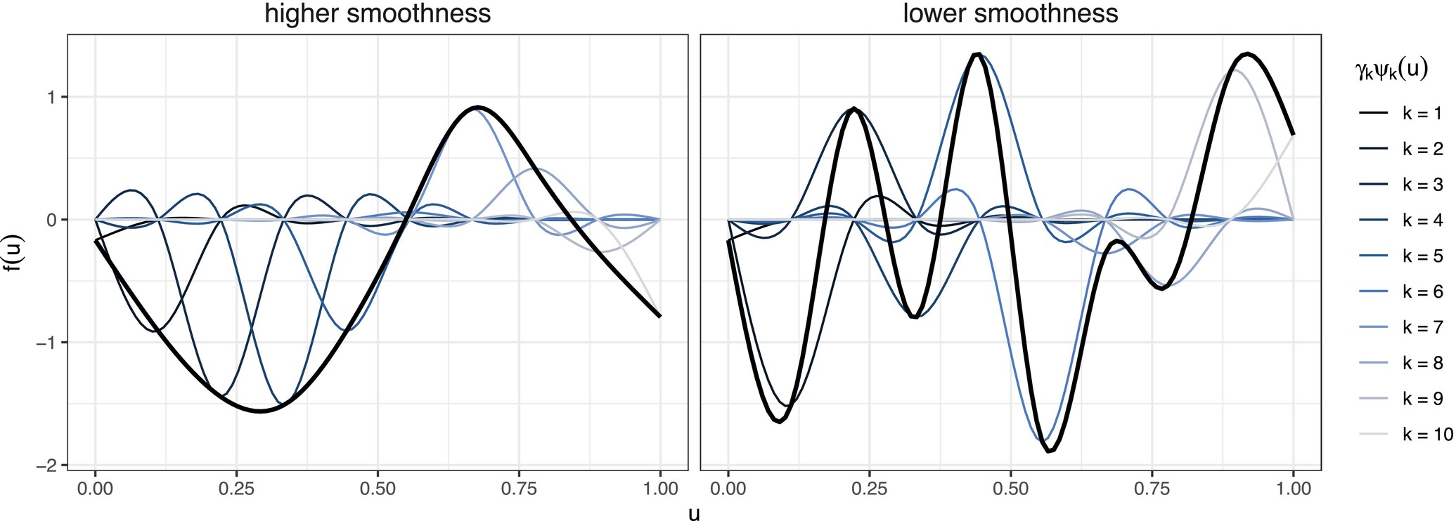
Smoothing splines
Loess (locally weighted linear regression)
Smoothing or Penalized Splines
Smoothing splines: Use lots of knots, but then attempt to balance overfitting and smoothness by controlling the size of the spline coefficients.
Klappstein, N. J., Michelot, T., Fieberg, J., Pedersen, E. J., & Mills Flemming, J. (2024). Step selection functions with non‐linear and random effects. Methods in ecology and evolution, 15(8), 1332-1346.
Other considerations
What if you want to allow for multiple non-linear relationships?
ns(x1, 3) + ns(x2, 4) or multiple smoothing splines
Other basis functions can be used to fit “smooth surfaces” (allowing for interactions between variables)
tensor splines, thin plate splines, etc…
Can include interactions (separate smooth for each level of a categorical variable)
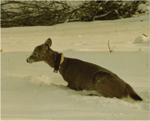
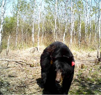
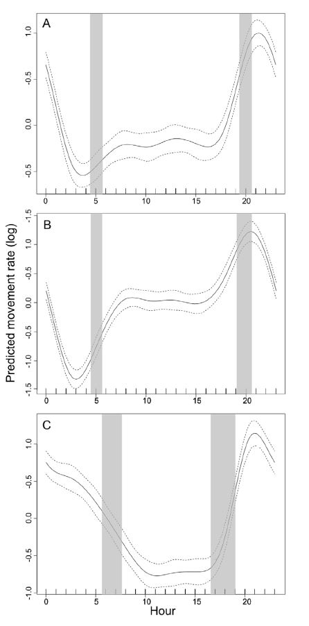
Black Bear Movement and Heart Rates
There are cyclical splines that
ensure ends meet at 0 and 24 hours
(or, Jan 1 and Dec 31).
Non-Linear Models with Mechanistic Basis
\(Y \sim f(x,\beta)\), where \(f(x,\beta)\) may have a strong theoretical motivation.
Ricker model for stock-recruitment: \(S_{t+1} = S_te^{r(1-\beta S_t)}\)
Predator prey: \(f(N) = \frac{aN}{1+ahN}\)
We will eventually learn how to fit these models using Maximum likelihood and Bayesian methods.