males<-c(120, 107, 110, 116, 114, 111, 113, 117, 114, 112)
females<-c(110, 111, 107, 108, 110, 105, 107, 106, 111, 111)
jawdat <- data.frame(jaws = c(males, females),
sex = c(rep("M",10), rep("F", 10)))Generalized Least Squares
FW8051 Statistics for Ecologists
Learning Objectives
Learn how to use Generalized Least Squares (GLS) to model data where \(Y_i|X_i\) is normally distributed, but the variance is not constant and may depend on one or more predictor variables.
GLS can also be used to model data that are correlated:
- Multiple measurements on the same sample unit (Chapter 18)
- Temporal dependence (Chapter 6 of Zuur et al)
- Spatial dependence (Chapter 7 of Zuur et al)
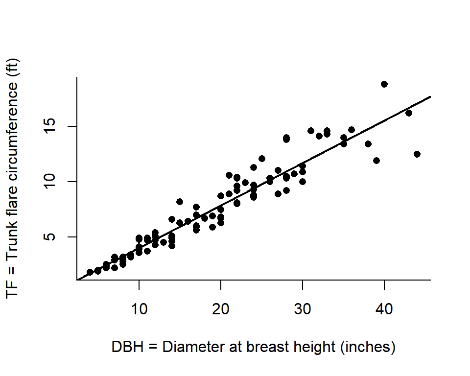
Trunk Flare Diameter
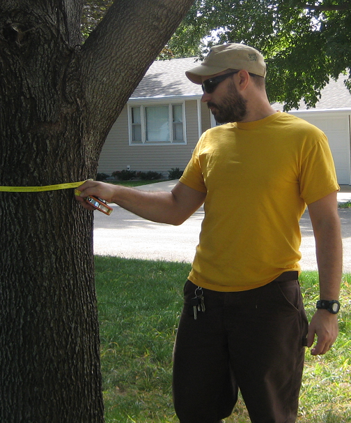
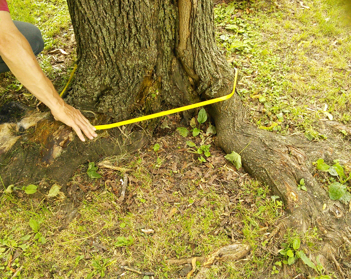
Eric North, PhD (former FW8051 student and urban forester).
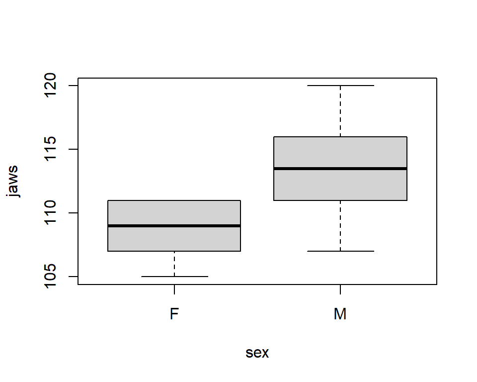
T-test with unequal variances: Jaw data
Linear Model
\(Y_i = \beta_0 + X_i\beta_1 + \epsilon_i\)
Assume \(\epsilon_i\) are independent, normally distributed, with constant variance.
\(\epsilon_i \stackrel{iid}{\sim} N(0, \sigma^2)\)
\(iid\) = independent and identically distributed
\[Y_i \sim N(\mu_i, \sigma^2)\]
\[\mu_i= \beta_0 + X_i\beta_1\]
Generalized Least Squares: Non-Constant Variance
\[Y_i \sim N(\mu_i, \sigma_i^2)\]
\[\mu_i= \beta_0 + X_i\beta_1\]
\[\sigma^2_i \sim f(X_i; \tau)\]
Model the mean and variance:
- \(\mu_i = \beta_0 + X_i\beta_1\)
- \(\sigma^2_i = f(X_i; \tau)\), where \(\tau\) are additional variance parameters.
Generalized Least Squares: Non-Constant Variance
\[Y_i \sim N(\mu_i, \sigma_i^2)\]
\[\mu_i= \beta_0 + X_i\beta_1\]
\[\sigma^2_i \sim f(X_i; \tau)\]
- the variance depends on the level of a categorical variable, \(g\)
varIdent: \(\sigma^2_i = \sigma^2_g\)
- the variance scales with a continuous covariate, \(X\)
varFixed: \(\sigma^2_i = \sigma^2X_i\)varPower: \(\sigma^2 |X_i|^{2\delta}\)varExp: \(\sigma^2e^{2\delta X_i}\)varConstPower: \(\sigma^2 (\delta_1 + |X_i|^{\delta_2})^2\)
- the variance depends on the mean
varPower(form = ~ fitted(.)): \(\sigma^2_i= \sigma^2\mu_i^{2\theta} = \sigma^2(\beta_0 + X_{1i}\beta_1 + X_{2i}\beta_2 + \ldots X_{pi}\beta_p)^{2\theta}\)
Interpretation
Many of these options can be understood in terms of a model for log(\(\sigma_i\))1:
varPower: \(\sigma^2_i = \sigma^2 |X_i|^{2\delta}\) \(\Rightarrow \log(\sigma_i) = log(\sigma) + \delta\log(|X_i|)\)
Notes:
- this takes the form \(y = mx + b\) with \(y = \log(\sigma_i), b = log(\sigma), m = \delta, x = log(|X_i|)\)
- log transformation ensures that \(\hat{\sigma}_i \ge 0\) (since \(\exp(x)\) is always > 0!)
varExp: \(\sigma^2_i = \sigma^2e^{2\delta X_i}\) \(\Rightarrow log(\sigma_i) = log(\sigma) + \delta X_i\)
- Again, takes the form \(y = b + mx\) with \(y = \log(\sigma_i), b = log(\sigma), m = \delta, x = X_i\)
We are assuming the log of the variance depends linearly on (\(X_i\)) or log(\(X_i\))
Other notes
One of my goals in this section is to demonstrate how we can fit flexible models formulated using:
- a statistical distribution (here, a Normal distribution)
- expressing parameters (here, \(\mu\) AND \(\sigma\)) of the distribution as a function of explanatory variables
Eventually, you will be able to formulate and fit custom models using Maximum Likelihood and Bayesian methods:
\[\sigma^2_i = \sigma^2 |X_i|^{2\delta_1}|Z_i|^{2\delta_2}\]
where \(X_i\) and \(Z_i\) are two different covariates and \(\sigma^2, \delta_1, \delta_2\) are parameters to be estimated.
T-test with unequal variances: Jaw data

T-test with unequal variances: Jaw data
\(Y_i\) = jaw length for jackal \(i\)
\[\begin{gather} Y_i \sim N(\mu_{i}, \sigma^2_{i}) \\ \mu_i = \beta_0 + \beta_1 \text{I(sex=male)}_i \\ \sigma_i^2 = \sigma^2_{sex} \end{gather}\]
Estimates of regression parameters are obtained by minimizing:
\[\begin{gather} \sum_{i = 1}^n \frac{(Y_i - \mu_i)^2}{2\sigma^2_i} \nonumber \end{gather}\]
Generalized least squares fit by REML
  Model: jaws ~ sex
  Data: jawdat
       AIC      BIC    logLik
  102.0841 105.6456 -47.04206

Variance function:
 Structure: Different standard deviations per stratum
 Formula: ~1 | sex
 Parameter estimates:
        M         F
1.0000000 0.6107279

Coefficients:
            Value Std.Error   t-value p-value
(Intercept) 108.6 0.7180211 151.24903  0.0000
sexM          4.8 1.3775993   3.48432  0.0026

 Correlation:
     (Intr)
sexM -0.521

Standardized residuals:
        Min          Q1         Med          Q3         Max
-1.72143457 -0.70466511  0.02689742  0.76657633  1.77522940

Residual standard error: 3.717829
Degrees of freedom: 20 total; 18 residual
Summary output
Apparent parameterization:
\(\sigma^2_{sex} = \sigma^2\delta^2_{sex}\), which is the same as \(\sigma_{sex} = \sigma\delta_{sex}\)
with:
- \(\hat{\delta}_{males}=1\)
- \(\hat{\delta}_{females} = 0.61\)
- \(\hat{\sigma} = 3.72\) (residual standard error)
Actual Parameterization
Actual parameterization used by R (linear model on log scale):
\(log(\sigma_i) = log(\sigma) + log(\delta)\text{I(sex = female)}_i\)
Ensures that \(\sigma_i\) is positive when we back-transform using exp().
\(\sigma_i = \sigma \delta^{\text{I(sex=female)}}\)
(see book for details if you are interested)
Fraser River Sockeye
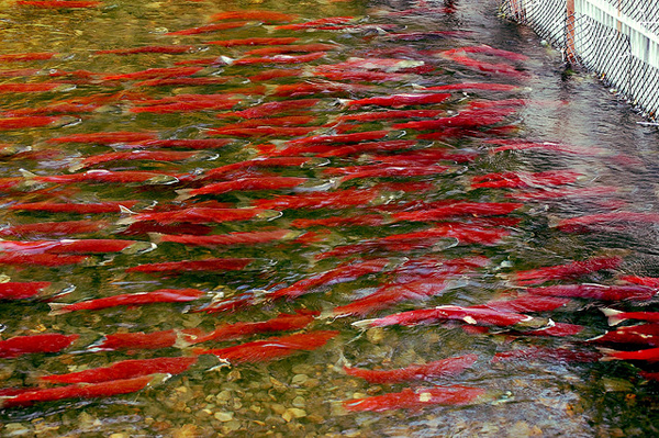
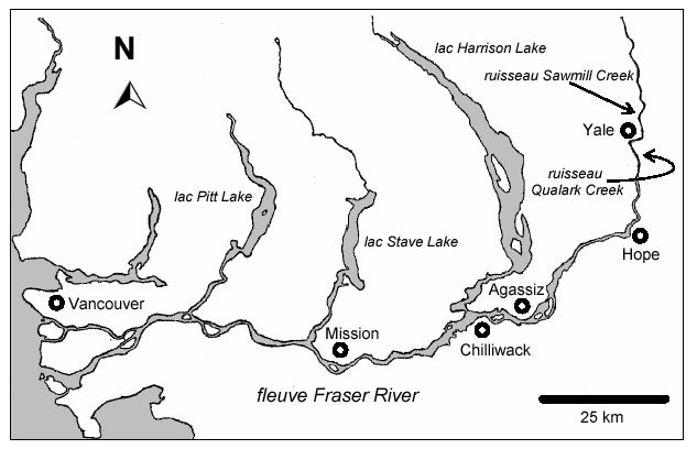
Use historical correlation between the count at Mission and \(S_t + C_t\) to manage the fishery
Variance increasing with \(X_i\) or \(\mu_i\)
- Fixed variance model: \(\sigma^2_i = \sigma^2\text{MisEsc}_i\)
- Power variance model: \(\sigma^2_i = \sigma^2|\text{MisEsc}_i|^{2\delta}\)
- Exponential variance model: \(\sigma^2_i = \sigma^2e^{2\delta \text{MisEsc}_i}\)
- Constant + power variance model: \(\sigma^2_i = \sigma^2(\delta_1 + |\text{MisEsc}_i|^{\delta_2})^2\)
See the book for syntax associated with the other models.
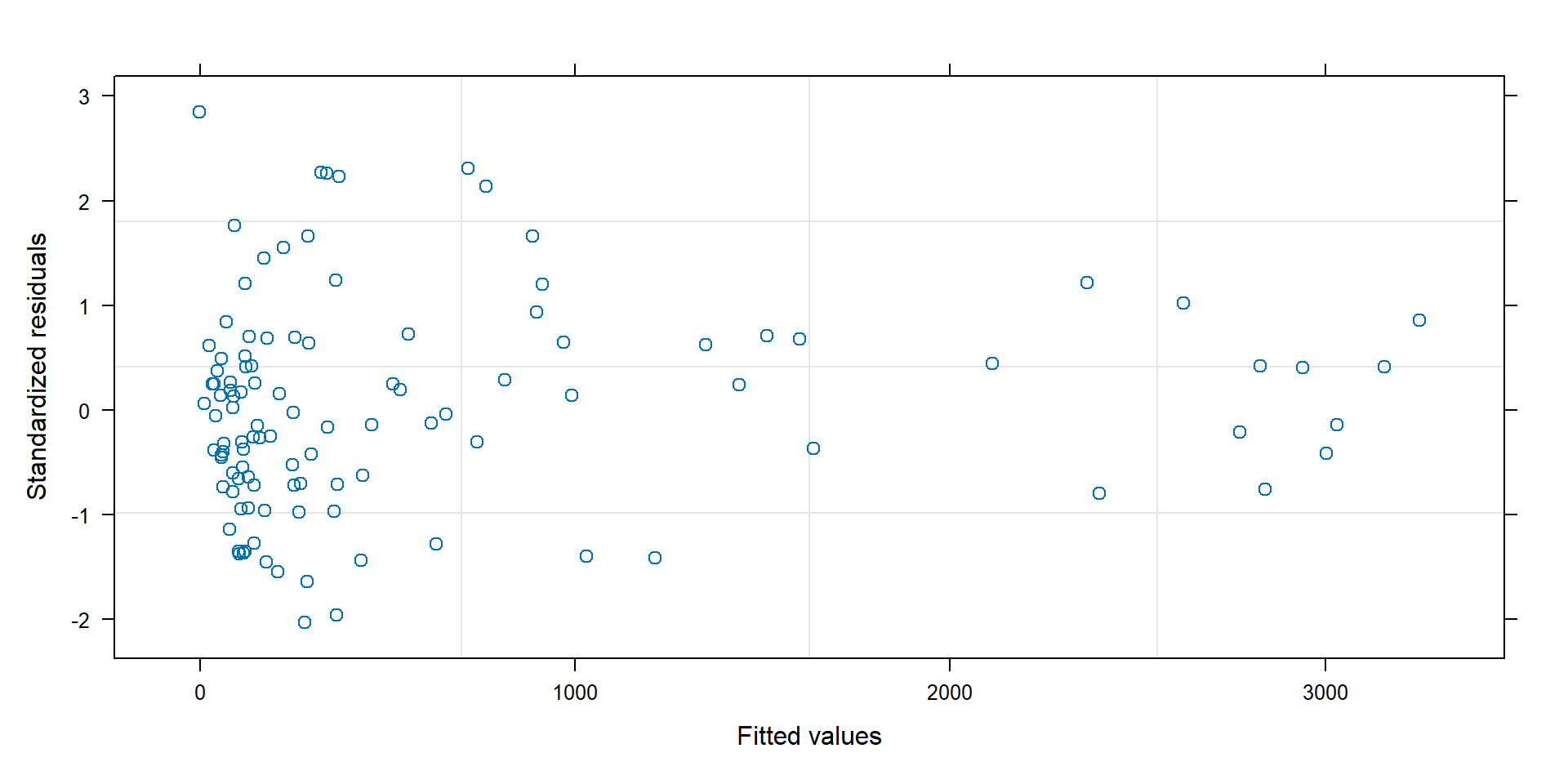
Standardized residuals
Standardized residuals = \((Y_i - \hat{Y}_i)/\hat{\sigma}_i\), should have approximately constant variance:

Variance depending on \(\mu_i\)
\[\begin{gather} Y_i \sim N(\mu_i, \sigma_i^2) \nonumber \\ \mu_i = \beta_0 + \beta_1X_i \nonumber \\ \sigma^2_i = \mu_i^{2\delta} \nonumber \end{gather}\]
Fit using varPower(form = ~ fitted(.)). See textbook via this link.
Selecting an appropriate variance model
- Plot residuals versus each predictor to see if the variance depends on a specific predictor
varPower(form = ~ fitted(.))can allow the variance to depend on multiple predictor variables since \(\sigma_i^2 = \sigma^2|\mu_i|^{2\theta}\), with \(\mu_i = \beta_0 + \beta_1X_{1i} + \ldots \beta_pX_{pi}\)- AIC can be used to compare multiple variance models, particularly if the variance part of the model is not of primary interest (e.g., we are just looking for more robust inference)
- Plot stanardized residuals: \((Y_i - \hat{\mu}_i)/\hat{\sigma}_i\) versus \(\hat{\mu}_i\). If the variance model is appropriate, these should have constant variance.
Zuur et al.’s Strategy (Section 4.2.3)
- Start with a “full model” (containing as many predictors as possible) fit using
gls
Inspect residuals, consider alternative variance structures if necessary (e.g., comparing models using AIC)
Settle on optimal variance model
- Choose best set of predictor variables for the mean of \(Y_i\) (using the variance model, chosen above)
- Check diagnostics again and pick best model
Approximate Confidence and Prediction Intervals
For a confidence interval, we need to consider:
\(var(\hat{\mu}_i) = var(\hat{\beta}_0 + X_i\hat{\beta}_1)\)
For a prediction interval, we need to consider:
\(var(\hat{Y}_i) = var(\hat{\beta}_0 + X_i\hat{\beta}_1+ \epsilon_i)\)
- Confidence interval = captures uncertainty regarding the average value of \(Y\) (given by the line)
- Prediction interval = captures uncertainty regarding a particular value of \(Y\) (need to also consider spread about the line)
Matrix Multiplication: Expected Value
\(\hat{\mu}_i = \hat{\beta}_0 + \hat{\beta_1}X_i\)
\(\hat{\mu}= \begin{bmatrix} 1 & X_1\\ 1 & X_2\\ \vdots & \vdots\\ 1 & X_n\\ \end{bmatrix}\begin{bmatrix} \hat{\beta}_0\\ \hat{\beta}_1\\ \end{bmatrix}=\begin{bmatrix} \hat{\beta}_0 + X_1\hat{\beta}_1\\ \hat{\beta}_0 + X_2\hat{\beta}_1\\ \vdots \\ \hat{\beta}_0 + X_n\hat{\beta}_1\\ \end{bmatrix}\)
Matrix multiplication: Variances
\(var(\hat{\mu}) = Var(\hat{\beta}_0 + X\hat{\beta}_1) = Var(\hat{\beta}_0) + X^2Var(\hat{\beta}_1)+2XCov(\hat{\beta}_0, \hat{\beta}_1)\)
Define:
Let \(X\) = \(\begin{bmatrix} 1 & X_1\\ 1 & X_2\\ \vdots & \vdots\\ 1 & X_n\\ \end{bmatrix}\) and \(X^\prime\) be its transpose
\(\hat{\Sigma} =\begin{bmatrix} \hat{\sigma}^2_{\hat{\beta}_0} & \hat{\sigma}^2_{\hat{\beta}_0,\hat{\beta}_1}\\ \hat{\sigma}^2_{\hat{\beta}_0,\hat{\beta}_1} & \hat{\sigma}^2_{\hat{\beta}_1} \\ \end{bmatrix}\)
\(\widehat{var}(\hat{\mu}) = Var(\hat{\beta}_0 + \hat{\beta}_1X)\) = \(X\hat{\Sigma}X^\prime\)
Calculations in R
We can use matrix multiplication to efficiently calculate intervals for multiple observations.
In R, we do this by using %*%
Let \(X\) = design matrix = \(\begin{bmatrix} 1 & X_1\\ 1 & X_2\\ \vdots & \vdots\\ 1 & X_n\\ \end{bmatrix}\)
\(\hat{\mu} = X\)%*% coef(modelname) gives us predicted values for all rows of the \(X\) matrix.
Calculations in R
\(\widehat{var}(\hat{\mu}) = X\)%*% vcov(modelname) %*%\(t(X)\)
vcov(model)= \(\hat{\Sigma}\) = estimated variance-covariance matrix of \(\hat{\beta}\) (works forlm,gls, maybe others)- We use
tto get a transpose of a matrix
We end up with a matrix that looks something like:
\(\begin{bmatrix} var(\hat{\mu}_1) & cov(\hat{\mu}_1, \hat{\mu}_2) & \cdots & cov(\hat{\mu}_1, \hat{Y}_n)\\ cov(\hat{\mu}_2, \hat{\mu}_1) & \ddots & \ddots & \vdots\\ \vdots & \ddots & \ddots & cov(\hat{\mu}_{n-1}, \hat{\mu}_n) \\ cov(\hat{\mu}_n, \hat{\mu}_1) & \cdots & cov(\hat{\mu}_{n}, \hat{\mu}_{n-1}) & var(\hat{\mu}_n)\\ \end{bmatrix}\)
Pull off the diagonal elements (the variances) - see the textbook for code.
Prediction Intervals
\(var(\hat{Y}_i) = var(\hat{\beta}_0 + X_i\hat{\beta}_1+ \epsilon_i)\)
- \(var(\epsilon_i) = \sigma^2_i\) and estimated by \(\hat{\sigma}^2_i\).
- In many cases, \(\hat{\sigma}^2_i\) is independent of \(\begin{bmatrix}\hat{\beta}_0 & \hat{\beta}_1\\ \end{bmatrix}\)
- This implies \(cov(\hat{\sigma}^2_i, \hat{\beta}_0) = cov(\hat{\sigma}^2_i, \hat{\beta}_1)=0\)
So, to construct a prediction interval, we approximate \(var(\hat{Y}_i)\) with:
\(\widehat{var}(\hat{Y}_i) \approx \widehat{var}(\hat{\beta}_0 + X_i\hat{\beta}_1) + \hat{\sigma}^2_i\) = \(X_i\hat{\Sigma}X_i^{\prime} + \hat{\sigma}^2_i\).
Additional Notes
Note, these estimates are approximate in that:
- They rely on asymptotic normality (central limit theorem) [think difference between \(t\) and \(z\)]
- They ignore uncertainty in the variance parameters