Understanding and Dealing with Collinearity
FW8051 Statistics for Ecologists
Learning Objectives: Collinearity
- What is collinearity/multicollinearity?
- How does one assess collinearity?
- What are the different types of collinearity?
- What are the effects of collinearity on
- Parameter estimates
- Standard errors
Will draw from:
- A lecture by Todd Steury, Auburn University
What is Collinearity?
Collinearity - when one predictor variable is correlated with another predictor variable.
Multicollinearity - when multiple predictor variables are correlated with each other.
Multicollinearity implies one of the explanatory variables can be predicted by the others with a high degree of accuracy.
Different Types of Collinearity
Intrinsic collinearity: multiple variables measure the same inherent quantity
- Various morphometric measurements (all capture “size”)
Compositional variables: have to sum to 1 (the last category is completely determined by the others)
- e.g., percent cover of different habitat types.
- Structural collinearity: occurs when variables are measured on very different scales (e.g., \(X\), \(X^2\))
- Incidental collinearity: variables may have separate effects but happen to covary in the data set possibly due to small sample sizes
Examples of Collinearity
- Habitat attributes: riparian areas also tend to have thick understory cover
- Urban areas have lots of impervious surface, minimal forest cover, high density of humans
- Areas farther north tend to be colder, get more snow, less sunlight in winter.
- Breeding behaviors of endangered butterflies depend on time of day, temperature, light availability
[Think-pair-share] Do you have similar examples from your study systems?
Symptoms of Collinearity
- Variables may be significant in simple linear regression, but not in multiple regression
- Large standard errors in multiple regression models despite large sample sizes/high power
- Variables may not be significant in multiple regression, but multiple regression model (as whole) is significant (e.g., using the F-test at the bottom of regression output)
- Large changes in coefficient estimates between full and reduced models
Symptoms of Collinearity
Interpretation of \(\beta\) in a multiple regression:
- Expected change in \(Y\) as we change \(X\) by 1 unit, while holding all other predictor variables constant.
- When predictors are collinear, changes in \(X\) tend to occur with changes in other variables too (making \(\beta\) hard to estimate)
Variance Inflation Factors
Multicollinearity can be measured using a variance inflation factor (VIF)
\(VIF(\hat{\beta}_j) = \frac{1}{1-R^2_{x_j|x_1, ..., x_{j-1}, x_{j+1}, x_p}}\), where
\(R^2_{x_j|x_1, ..., x_{j-1}, x_{j+1}, x_p}\) = multiple \(R^2\) from: lm(\(x_j \sim x_1 + \ldots + x_{j-1} + x_{j+1} + x_p\))
If a variable can be predicted from the other variables in the regression model, then it will have a large VIF.
Calculate using the vif function in the car package
Rules of Thumb in Published Literature:
- Many suggest VIFs \(\ge 10\) are problematic
- Graham (2003): VIFs as small as 2 can have significant impacts
Sleep example
Look at sleep example from book.
Simulation study: Confounding Variables
Truth:
- \(Y_i = 10 + 3X_{1,i} + 3X_{2,i} + \epsilon_i\) with \(\epsilon_i \sim N(0,2)\)
- \(X_{1,i} \sim U(0,10)\)
- \(X_{2,i} =\tau X_{1,i} + \gamma_i\) with \(\gamma_i \sim N(0, 4)\)
- Varied \(\tau\) from 0 to 9 by 3 (
tau <- seq(0,9,3))
Simulated 2000 data sets and to each fit:
lm(Y ~ X1)lm(Y ~ X1+X2)
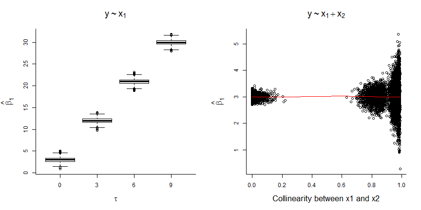
- coefficient for \(X_1\) is biased when \(X_2\) is not included (unless \(\tau=0\))
- magnitude of the bias increases with the correlation between \(X_1\) and \(X_2\) (i.e., with \(\tau\))
- coefficient for \(X_1\) is unbiased when \(X_2\) is included, but SE increases when \(X_1\) and \(X_2\) are highly correlated
Mathematically…
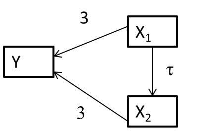
\[Y_i = 10 + 3X_{1,i} + 3X_{2,i} + \epsilon_i \text{ and } X_{2,i} =\tau X_{1,i} + \gamma_i\]
\[Y_i = 10 + 3X_{1,i} + 3(\tau X_{1,i} + \gamma_i) + \epsilon_i\]
\[Y_i = 10 + (3+3\tau)X_{1,i} + (3\gamma_i + \epsilon_i)\]
Causal Networks
- \(X_1\) captures the effect of both \(X_1\) and \(X_2\) when \(X_2\) is left out of the model!
- When we leave \(X_2\) out of the model, the coefficient for \(X_1\) captures the direct of effect of \(X_1\) on \(Y\) and also the indirect effect of \(X_1\) on \(Y\) (mediated by \(X_2\))
Trade-offs
Models with collinear variables
- Large standard errors
Models in which confounding variables are left out
- Misleading estimates of effect due to omission of important variables
When possible, try to eliminate confounding variables via study design (e.g., experiments, matching)
Strategies for dealing with multicollinearity
If the only goal is prediction, may choose to ignore multicollinearity
- Often has minimal impact on prediction error (versus SEs for individual coefficients)
- Can be problematic if making out-of-sample predictions where the extent and nature of collinearity changes
For estimation, there are methods that introduce some bias to improve precision
- Ridge regression, LASSO (ch 8)
Other methods
Graham (2003) and the textbook also briefly consider:
- Residual and sequential regression
- Principal component regression
- Structural equation models (related to causal inference methods in Ch 7)
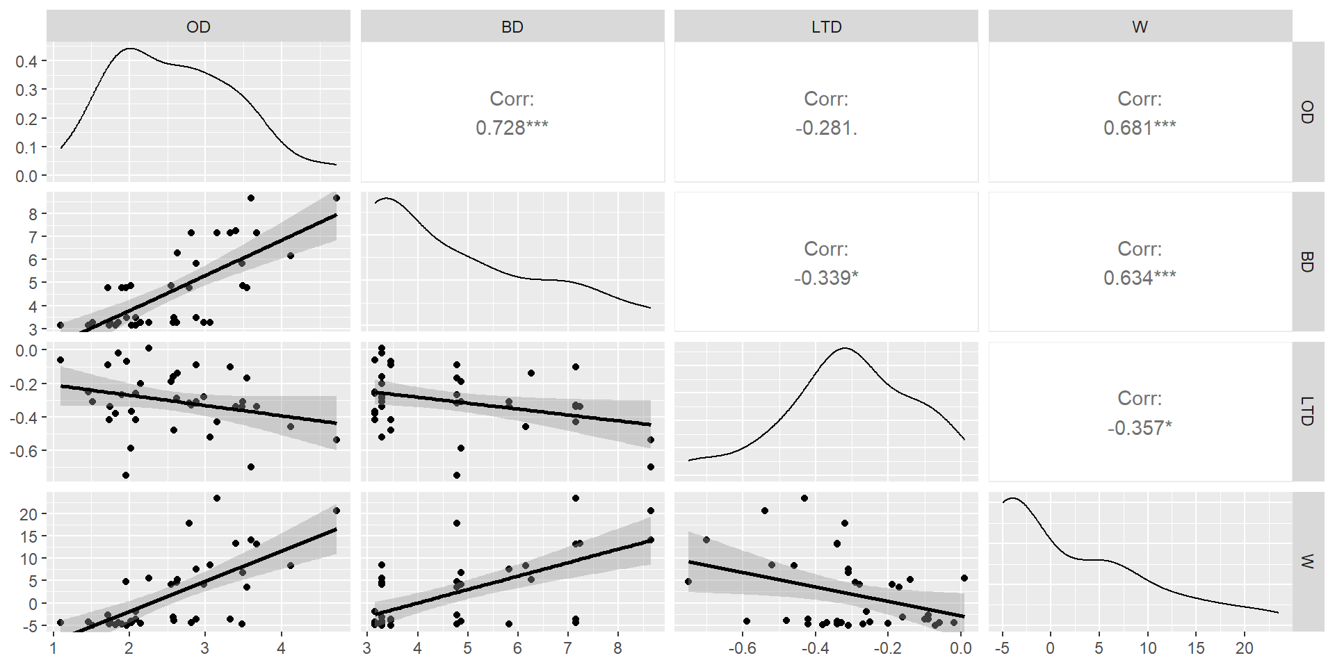
Example from Graham (2003):
- OD = wave orbital displacement (in meters)
- BD = wave breaking depth (in meters)
- LTD = average tidal height (in meters)
- W = wind velocity (in meters/s).
      OD       BD      LTD        W
2.574934 2.355055 1.175270 2.094319
Always look at the relationship among your predictors (without the response variables) as a first step to assessing collinearity!
Residual and sequential regression
Prioritize different variables to include sequentially:
- Include \(x_1\) (unique and shared contributions)
- Then, residuals of lm(\(x_2 \sim x_1)\) (part of \(x_2\) not shared with \(x_1\))
- Then, residuals of lm(\(x_3 \sim x_1 + x_2)\) (part of \(x_3\) not shared with \(x_1\) or \(x_2\))
- …
How to Prioritize?
- Instincts and intuition
- Previously collected data
Graham considered (newly formed) predictors in this order:
- OD = captures unique effect of OD + shared effect with other variables
- W|OD = captures effect of W not shared with OD
- LTD|OD, W = captures effect of LTD that is not shared with OD or W
- BD|OD, W, LTD = captures effect of BD not shared with OD, W, LTD
Call:
lm(formula = Response ~ OD + W.g.OD + LTD.g.W.OD + BD.g.W.OD.LTD,
    data = Kelp)

Residuals:
      Min        1Q    Median        3Q       Max
-0.284911 -0.098861 -0.002388  0.099031  0.301931

Coefficients:
               Estimate Std. Error t value Pr(>|t|)
(Intercept)    2.747588   0.078192  35.139  < 2e-16 ***
OD             0.194243   0.028877   6.726 1.16e-07 ***
W.g.OD         0.008082   0.003953   2.045   0.0489 *
LTD.g.W.OD    -0.055333   0.141350  -0.391   0.6980
BD.g.W.OD.LTD -0.004295   0.021137  -0.203   0.8402
---
Signif. codes:  0 '***' 0.001 '**' 0.01 '*' 0.05 '.' 0.1 ' ' 1

Residual standard error: 0.1431 on 33 degrees of freedom
Multiple R-squared:  0.6006,    Adjusted R-squared:  0.5522
F-statistic: 12.41 on 4 and 33 DF, p-value: 2.893e-06 Estimate Std. Error t value Pr(>|t|)
(Intercept) 2.747587774 0.07819170 35.1391212 1.000393e-27
OD 0.194243475 0.02887749 6.7264678 1.156387e-07
W.g.OD 0.008082141 0.00395292 2.0446003 4.893874e-02
LTD.g.W.OD -0.055333263 0.14135008 -0.3914626 6.979717e-01
BD.g.W.OD.LTD -0.004294572 0.02113731 -0.2031750 8.402459e-01Residual and sequential regression
Advantages:
- Unique and shared contributions are represented in the model
- Decisions to include or exclude a variable will not depend on what other predictors are included in the model
Disadvantages:
- Requires prioritization (which may not be reflect functional importance of the variables)
Principal Components Regression
Form new predictors as linear combinations of the correlated variables:
\(pca_1 = \lambda_{1,1}X_1 + \lambda_{1,2}X_2 + \ldots \lambda_{1,p}x_p\)
\(pca_2 = \lambda_{2,1}X_1 + \lambda_{2,2}X_2 + \ldots \lambda_{2,p}x_p\)
\(\cdots\)
\(pca_p = \lambda_{p,1}X_1 + \lambda_{p,2}X_2 + \ldots \lambda_{p,p}x_p\), where
- The \(pca_i\)’s are all orthogonal (statistically independent)
- \(pca_1\) accounts for the greatest variation in \((x_1, x_2, ..., x_p)\)
- \(pca_2\) accounts for greatest amount of remaining variation in \((x_1, x_2, ..., x_p)\), not accounted for by \(pca_1\)
- …
           PC1        PC2         PC3         PC4
OD   0.5479919 -0.2901058 -0.15915149 -0.76825404
BD   0.5453470 -0.1793692 -0.58088137  0.57706165
LTD -0.3384653 -0.9335391  0.06706729  0.09720099
W 0.5364166 -0.1103180 0.79545560 0.25949479 OD BD LTD W PC1 PC2 PC3 PC4
1 2.0176 4.87 -0.59 -4.1 -0.19127827 1.7527358 -0.66278941 0.24694830
2 1.9553 4.78 -0.75 4.7 0.62234092 2.5023873 0.18091063 0.46900655
3 1.8131 3.14 -0.38 -4.9 -1.33268779 0.9190480 -0.03361542 -0.05590063
4 2.5751 3.28 -0.16 -3.2 -1.08056344 -0.5416139 0.01891911 -0.55322453
5 2.2589 3.28 0.01 5.6 -1.03524778 -1.4381622 1.00570204 0.11858908
6 2.5448 4.87 -0.19 4.1 -0.05452203 -0.6398905 0.18695547 0.22937274Biplot
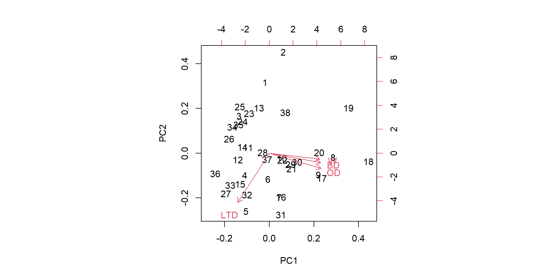
Principal Components Regression
Importance of components:
                          PC1    PC2     PC3     PC4
Standard deviation     1.6017 0.8975 0.60895 0.50822
Proportion of Variance 0.6413 0.2014 0.09271 0.06457
Cumulative Proportion  0.6413 0.8427 0.93543 1.00000
The first principal component explains 64% of the variation in (OD, BD, LTD, W)
Choose one or more \(pca_i\) to include as new regressors (Graham 2003 suggests including all of them).
- \(pca_1\) explains the greatest variation in \((x_1, x_2, ..., x_p)\) (not necessarily the greatest variation in \(Y\))
- Since the \(pca_i\)’s are orthogonal, the coefficients will not change as other \(pca_i\)’s are added or dropped.
Principal Components Regression
Call:
lm(formula = Response ~ PC1 + PC2 + PC3 + PC4, data = Kelp)

Residuals:
      Min        1Q    Median        3Q       Max
-0.284911 -0.098861 -0.002388  0.099031  0.301931

Coefficients:
            Estimate Std. Error t value Pr(>|t|)
(Intercept)  3.24984    0.02321 140.035  < 2e-16 ***
PC1          0.09806    0.01468   6.678 1.33e-07 ***
PC2         -0.02971    0.02620  -1.134    0.265
PC3          0.03612    0.03862   0.935    0.356
PC4         -0.07826    0.04628  -1.691    0.100
---
Signif. codes:  0 '***' 0.001 '**' 0.01 '*' 0.05 '.' 0.1 ' ' 1

Residual standard error: 0.1431 on 33 degrees of freedom
Multiple R-squared:  0.6006,    Adjusted R-squared:  0.5522
F-statistic: 12.41 on 4 and 33 DF,  p-value: 2.893e-06
Principal Components Regression
The main disadvantage is the principal components can be difficult to interpret.
Options:
- Can apply separately to groups of like variables (“weather”, “vegetation”, etc)
- Consider other “rotations” (that ensure that some \(\lambda_{i,j} = 0\))
- Other variable clustering methods that group variables (Harrell 2001. Regression Modeling Strategies).
Structural Equation Modeling
- Chapter on Causal Models (on Moodle)
- Allows for direct and indirect effects
- Can account for unique and shared contributions (the latter through latent variables)
- Focuses on a priori modeling and testing of hypothesized relationships
Conclusions from Graham (2003)
“The suite of techniques described herein compliment each other and offer ecologists useful alternatives to standard multiple regression for identifying ecologically relevant patterns in collinear data. Each comes with its own set of benefits and limitations, yet together they allow ecologists to directly address the nature of shared variance contributions in ecological data.”