Gain a deeper appreciation for why correlation (or association) is not the same as causation
Discover basic rules that allow one to determine dependencies (correlations) among variables from an assumed causal network
Understand how causal networks can be used to inform the choice of variables to include in a regression model
Causation versus correlation
Knowing what causes what makes a big difference in how we act. If the rooster’s crow causes the sun to rise we could make the night shorter by waking up our rooster earlier and make him crow - say by telling him the latest rooster joke. - Judea Pearl (1936-), computer scientist
Regression
Regression models describe correlations among explanatory (\(x_1, x_2, ...x_k\)) variables and a response variable (\(y\)).
These correlations depend on how the data were collected (e.g., experimental or observation data, the population that was sampled, etc).
Regression coefficients change depending on what other variables are included.
Regression and Causal Mechanisms
Often, we want to interpret models as capturing causal mechanisms so we can say what will happen if we intervene in the system:
Will taking a daily vitamin improve long-term health?
Will increasing the pay of teachers or reducing class size boost student performance?
Will increasing taxes on the rich cause companies to relocate?
Will we decrease deer population size if we institute an Earn-a-buck regulation?
Counterfactuals
We may also be interested in asking hypothetical questions. What would have happened if…
A judge may have to decide if a worker’s claim of sex discrimination is legitimate: would the worker have gotten the job if she was a male?
The National Park Service commissioned a study to ask if fewer birds would have died from collisions had a bridge in Hastings MN been built differently.
These questions involve counterfactuals= something that did not happen, but would have happened if something had been different.
Correlations
Correlations by themselves are not sufficient for answering these questions.
Will taking a daily vitamin improve our long-term health?
People that take vitamins may have better health outcomes, but they may also…
Exercise more
Eat healthier
Drive more cautiously
Interventions: Direct and Indirect Effects
Changing one variable, may lead to changes in others…
If we increase taxes on the rich, can we predict whether businesses will leave the state?
Attractiveness to a business may depend on:
state taxes
school system in the state
Increasing taxes may allow a state to invest more in their schools.
direct effect (negative) due to increased taxes
indirect effect (positive) through improvement in schools
Predicting the effect of an intervention requires something more complex…
Campaign Spending: Correlation vs. Causation
Campaign spending data from US Congressional elections
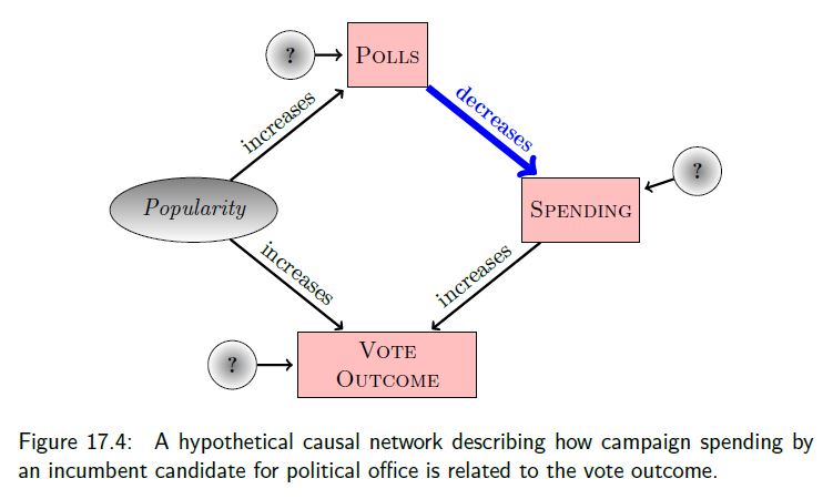
Increased spending by those running for re-election (incumbents) is associated with lower vote percentages
Why?
Causal network= Hypothetical model of how the system works
Nodes: represent variables or components in a system
Boxes = observed
Ellipses = not observed
Circles = random noise, suggests something outside of the system influences the variable
Links: connections between nodes
arrows = causal mechanistic connections
lines or double arrows = associations (non-causal links)
Using Simulation to Explore Campaign Spending
nsamps <-435# number of observationspopularity <-runif(nsamps, min=15, max=85)polls <- popularity +rnorm(nsamps, sd=3)spending <-100- polls +rnorm(nsamps,sd=10)vote <-0.75*popularity +0.25*spending +rnorm(nsamps,sd=5)votedat<-data.frame(popularity=popularity,polls=polls, spending=spending, vote=vote)
Call:
lm(formula = vote ~ spending + polls, data = votedat)

Residuals:
    Min      1Q  Median      3Q     Max
-15.468  -3.870   0.231   3.933  14.081

Coefficients:
            Estimate Std. Error t value Pr(>|t|)
(Intercept) -1.10903    2.87109  -0.386    0.699
spending     0.27282    0.02833   9.629   <2e-16 ***
polls        0.74546    0.03022  24.667   <2e-16 ***
---
Signif. codes:  0 '***' 0.001 '**' 0.01 '*' 0.05 '.' 0.1 ' ' 1

Residual standard error: 5.616 on 432 degrees of freedom
Multiple R-squared:  0.7791,    Adjusted R-squared:  0.7781
F-statistic: 761.9 on 2 and 432 DF,  p-value: < 2.2e-16
Consider the following DAG:
Code
DiagrammeR::grViz("digraph { graph [ranksep = 0.8] node [shape = box] A [label = 'Days Fishing'] B [label = 'Interest in Natural Resources'] C [label = 'St. Paul Courses'] D [label = 'Interest in Nutrition'] edge [minlen = 2] B -> A B -> C D -> C { rank = same; A; B }}")
I’ve simulated data using these assumptions (note interest in nutrition and fishing are not causally connected):
# Set seed of random number generatorset.seed(1040)# number of studentsn <-5000# Interest in nutrition sciencesnut <-runif(n, 0, 2)# Interest in natural resourcesnri <-runif(n, 0, 2)# Number of days fishingf <-rpois(n, lambda=2*nri)# Indicator variable (taking classes on St. Paul campus?)p <-exp(-5+2*nut +2*nri)/(1+exp(-5+2*nut +2*nri))z <-rbinom(n, 1, prob=p)# Create data setdagdata<-data.frame(nutrition.interest=nut, natresource.interest=nri, fishing=f, stpaulcampus=z)
Call:
lm(formula = fishing ~ nutrition.interest + stpaulcampus, data = dagdata)

Residuals:
    Min      1Q  Median      3Q     Max
-3.0785 -1.4643 -0.4563  1.1385  9.5828

Coefficients:
                   Estimate Std. Error t value Pr(>|t|)
(Intercept)         1.94570    0.05007  38.862  < 2e-16 ***
nutrition.interest -0.35380    0.04697  -7.532 5.91e-14 ***
stpaulcampus        1.13656    0.05715  19.887  < 2e-16 ***
---
Signif. codes:  0 '***' 0.001 '**' 0.01 '*' 0.05 '.' 0.1 ' ' 1

Residual standard error: 1.764 on 4997 degrees of freedom
Multiple R-squared:  0.07337,   Adjusted R-squared:  0.07299
F-statistic: 197.8 on 2 and 4997 DF,  p-value: < 2.2e-16
Confused?
In the first example, we got the ‘right answer’ when we adjusted for polls.
In the second example, adjusting for whether the student was taking courses on the St. Paul campus created a spurious (negative) correlation between interest in nurtition and fishing.
Should we adjust or not? It depends on one’s hypothetical model of the system (i.e., the causal network)!
Selection Bias
What happens if we only survey students on the St. Paul campus?
Selecting only individuals taking courses on the St. Paul campus has the same effect as adjusting for the variable in the regression.
Call:
lm(formula = fishing ~ nutrition.interest, data = subset(dagdata,
    stpaulcampus == 1))

Residuals:
    Min      1Q  Median      3Q     Max
-2.9047 -1.5545 -0.4951  1.3329  9.5089

Coefficients:
                   Estimate Std. Error t value Pr(>|t|)
(Intercept)         2.90711    0.12682  22.924   <2e-16 ***
nutrition.interest -0.22129    0.08956  -2.471   0.0136 *
---
Signif. codes:  0 '***' 0.001 '**' 0.01 '*' 0.05 '.' 0.1 ' ' 1

Residual standard error: 1.889 on 1721 degrees of freedom
Multiple R-squared:  0.003535,  Adjusted R-squared:  0.002956
F-statistic: 6.105 on 1 and 1721 DF,  p-value: 0.01357
Causal network or Directed Acyclical Graph
Causal network= Hypothetical model of how the system works
We will not consider (closed loops): \(C \rightarrow B \rightarrow A \rightarrow C\) which raise questions of “when”
\(A \Leftrightarrow B\) means that there is a non-causal connection between \(A\) and \(B,\) usually due to an unobserved variable, \(U\), responsible for the correlation.
Direct, indirect, and total effects
A direct effect is one that is represented by a path between two nodes (without consideration of any intermediate nodes): \(C \rightarrow A\)
An indirect effect is one that connects two nodes, but where we also consider an intermediate node: \(C \rightarrow B \rightarrow A\). Here, \(B\) is a called a mediator variable.
The total effect is the sum of direct and indirect effects
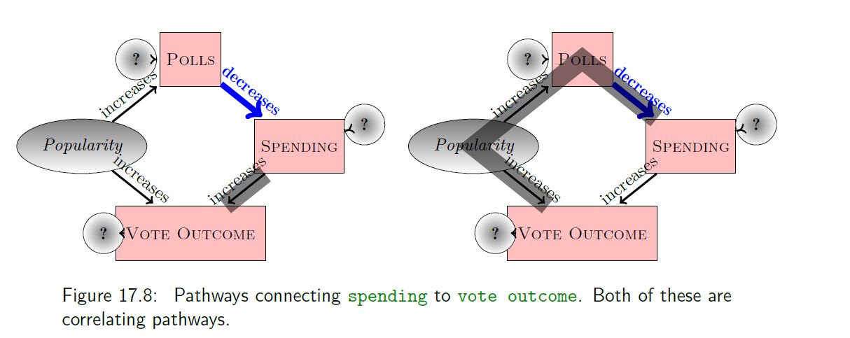
Pathways
A pathway between two nodes is a route between them (may pass through other nodes along the way)
\(A\) = a response variable
\(B\) = an explanatory variable
\(C\) = a covariate
Causal mediator: \(B \rightarrow C \rightarrow A\)
Common cause or confounder: \(B \leftarrow C \rightarrow A\)
Common effect or collider: \(B \rightarrow C \leftarrow A\)
Pathways
A pathway between two variables (\(A\) and \(B\)) is correlating if there is a node on the pathway from which you can get to both variables.
Causal mediator: \(B \rightarrow C \rightarrow A\) (correlating)
Common cause: \(B \leftarrow C \rightarrow A\) (correlating)
Witness: \(B \rightarrow C \leftarrow A\) (non-correlating)
“Correlating” implies that the variables \(A\) and \(B\) will be associated (if we do not consider or adjust for the variable \(C\)).
What about \(B \rightarrow C \rightarrow D \rightarrow A\)? Correlating!
“Adjusting” for the variable \(C\)
Causal mediator: \(B \rightarrow C \rightarrow A\)
Including \(C\)blocks the pathway, which is otherwise open (i.e., correlating)
Common cause: \(B \leftarrow C \rightarrow A\)
Including \(C\)blocks the pathway, which is otherwise open (i.e., correlating)
Witness: \(B \rightarrow C \leftarrow A\)
Including \(C\)opens the pathway, which is otherwise blocked.
Good versus bad controls
To identify which variables to include when estimating the causal effect of \(B\) on \(A\):
Write down all paths connecting \(B\) and \(A\)
Identify the path(s) you are interested in quantifying (this depends on whether you are interested in direct or total effects)
Block any other correlating paths (e.g., by including “good” controls)
Make sure NOT to unblock closed paths by including collider/common effects (i.e., “bad” controls)
Back to Polls
And fishing/nutrition example
Estimates of Direct and Indirect Effects
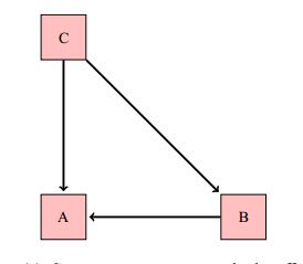
What if we want to estimate the direct effect of C on A?
Pathways:
\(C \rightarrow A\) (correlating), and the effect of interest.
\(C \rightarrow B \rightarrow A\) (correlating), an indirect effect of \(C\) on \(A\) that is mediated by \(B\)
Include \(B\) to block!
lm(A \(\sim\)C + B)
Estimates of Direct and Indirect Effects
What if we want to estimate the totol effect of C on A?
Pathways:
\(C \rightarrow A\) (correlating)
\(C \rightarrow B \rightarrow A\) (correlating)
In this case, we would not want to include B as it would block the second pathway representing an indirect effect of \(C\) on \(A\).
lm(A \(\sim\)C)
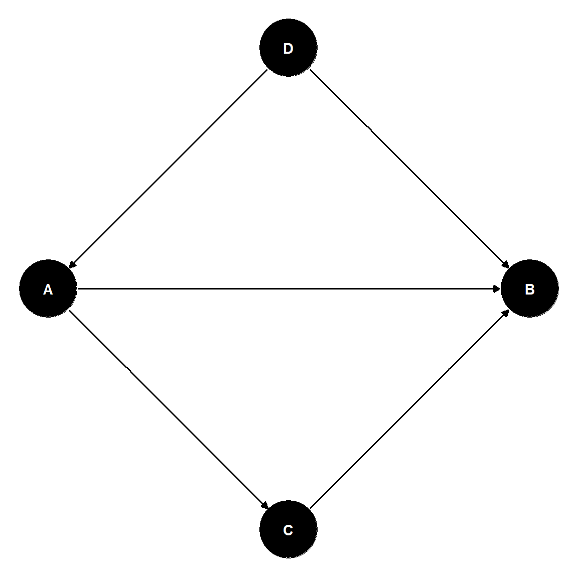
Pathways and Choice of Covariates
Goal: study the direct effect of \(A\) on \(B\).
Pathways and Choice of Covariates
Pathways:
\(A \rightarrow B\)
(correlating), effect of interest.
\(B \leftarrow D \rightarrow A\)
(correlating) Include D to block!
\(A \rightarrow C \rightarrow B\)
(correlating) Include \(C\) to block!
lm(B \(\sim\)A + C + D)
To study the total effect of \(A\) on \(B\), we would use:
lm(B \(\sim\)A + D).
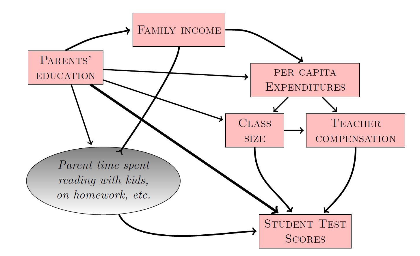
Student Test Scores
Effect of per-captita expenditures on Student Test Scores:
Include Class Size?
Include Teacher Compensation?
(No and No)
Per-captia expenditures \(\rightarrow\) (Class Size, Teacher Compensation) \(\rightarrow\) Test Scores
Student Test Scores
Include Parents’ Education?
Per-capita expenditures \(\leftarrow\) Parents’ education \(\rightarrow\) Test scores
Include Parents’ education to block the path!
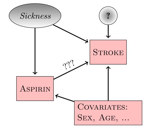
Experiments
If we can’t measure “sickness”, we can’t block the backdoor path (Aspirin \(\leftarrow\) Sickness \(\rightarrow\) Stroke)
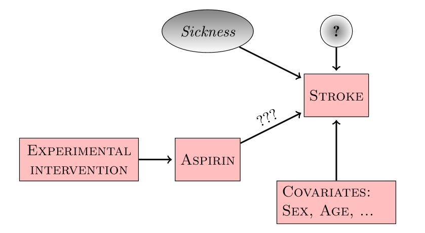
Experiments revisited
Randomly assigning aspirin (treatment) eliminates the connection between Sickness and Aspirin!
Summary
Causal networks / Directed acyclical graphs (DAGs) provide a better rational for including/excluding variables than p-values, AIC, etc when the goal is to understand causal mechanisms.
They can also help understanding why:
coefficients change (possibly even their sign) when we include or exclude other explanatory variables
experiments are the gold standard for inferring causality