Multi-Model Inference
Learning objectives
Gain an appreciation for challenges associated with selecting among competing models and performing multi-model inference.
Understand common approaches used to select a model (e.g., stepwise selection using p-values, AIC, Adjusted \(R^2\)).
Understand the implications of model selection for statistical inference.
Gain exposure to alternatives to traditional model selection, including full model inference (df spending), model averaging, and penalized likelihood/regularization techniques.
Be able to evaluate evaluate model performance using cross-validation and model stability using the bootstrap.
Be able to choose an appropriate modeling strategy, depending on the goal of the analysis (describe, predict, or infer).
Goals of multivariable regression modeling
- Describe: capture the main features of the data in a parsimonious way; which factors are related to the response variable and how?
- Explain: test and compare existing theories about which variables, or combination of variables, are causally related to the response variable. Regression coefficients should ideally capture how each variable affects the response variable.
- Predict: Use a set of sample data to make predictions about future data. It will be important to consider causality/confounding when making predictions for new populations (e.g., new spatial locations).
My Experience
Linear Models Mid-term
- Asked to develop a predictive model of Serum Albumin levels
- Given real data set (lots of predictors, missing data, etc)
- Given a weekend to complete the analysis and write up our report
Goals were largely to demonstrate:
- Knowledge of linear models (diagnostics, model selection, etc)
- Ability to generate reliable inference
Strategy I took:
- \(n = 136\) observations, split 80% (training data) and 20% (test data)
- Did lots of stuff w/ the training data
- Grouped variables into similar categories (e.g., socio-economic status, stature [height, weight, etc], dietary intake variables)
- Examined variables for collinearity and tried to pick the best one in a group using all possible regressions involving the group of variables
- Fit a “best model”, considered diagnostics (normality, constant variance, etc), then looked to see if any important variables were omitted
- Grouped variables into similar categories (e.g., socio-economic status, stature [height, weight, etc], dietary intake variables)
- Used the test data to evaluate predictive ability
Results
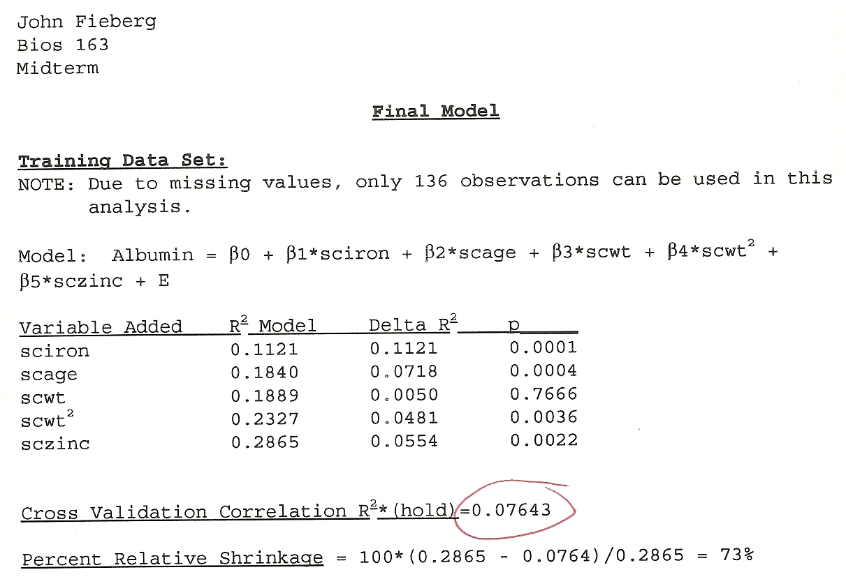
Figure 1: My mid-tem exam from my Linear Models class.
Traditional approaches used to compare models
Nested and Non-nested Models
Nested = can get from one model to the other by setting one or more parameters = 0.
- \(\mbox{Sleep} = \beta_0 + \beta_1\mbox{Danger} + \beta_2\mbox{LifeSpan}\)
- \(\mbox{Sleep} = \beta_0 + \beta_1\mbox{Danger}\)
Model comparisons
We can compare nested models using…
- p-values from hypothesis tests (nested models only), t-tests, F-tests, likelihood ratio tests
And, nested or non-nested models using…
- Compare adjusted \(R^2\) between competing models
- Compare model AIC values = -2*log-likelihood + 2p (nested and non-nested models; smaller is better)
Problem 1: different (arbitrary) criteria often point to different models as “best.”
Problem 2: the importance of a variable may depend on what else is in the model!
How do we choose a best model?
If we have several potential predictors, how can we decide on a best model?
- We can compare a list of nested models in a structured way (adding variables or deleting variables using “stepwise selection” procedures)
- We can compare any list of models (nested or non-nested) using AIC
- We can “think hard” about the problem and focus on a single most appropriate model (with others models considered as part of a “sensitivity analysis”)
Modeling Strategies
Stepwise Variable Selection
One method: Backward Elimination
- Start with a model with multiple predictors
- Consider all possible models formed by dropping 1 of these predictors
- Keep the current model, or drop the “worst” predictor depending on:
- p-values from the individual t-tests (drop the variable with the highest p-value, if \(>0.05\))
- Adjusted \(R^2\) values (higher values are better)
- AIC (lower values are better)
- Rinse and repeat until you can no longer improve the model
The stepAIC function in the MASS library will do this for us.
Can also do “forward selection” (or fit all possible models “all subsets”)
Change-in-estimate criterion
Heinze et al. (2017) suggest using “augmented backwards elimination”
Eliminate variables using significant testing, but only drop a variable if it does not lead to large changes in other regression coefficients.
Available in abe package (I have not used, but am intrigued…)
Data-Driven Inference
Problem 4: p-values, confidence intervals, etc assume the model has been pre-specified. Measures of fit, after model selection, will be overly optimistic.
Problem 5: no guarantee that the ‘best-fit’ model is actually the most appropriate model for answering your question.
Stepwise selection
Harrel et al. 2001. Regression Modeling Strategies:
- \(R^2\) values are biased high.
- The ordinary F and \(\chi^2\) test statistics do not have the claimed distribution
- SEs of regression coefficients will be biased low and confidence intervals will be falsely narrow.
- p-values will be too small and do not have the proper meaning (due to multiple comparison problems).
- Regression coefficients will be biased high in absolute magnitude.
- Rather than solve problems caused by collinearity, variable selection is made arbitrary by collinearity.
- It allows us not to think about the problem.
Stepwise Selection
Copas and Long,” the choice of the variables to be included depends on estimated regression coefficients rather than their true values, and so \(X_j\) is more likely to be included if its regression coefficient is over-estimated than if its regression coefficient is underestimated.”
Stepwise methods often select noise variables rather than ones that are truly important.
Problems get worse as you consider more candidate predictors and as these predictors become more highly correlated.
Regression Modeling Strategies (Frank Harrell’s book)
Why do variable selection?
- Desire to find a ‘concise’ model
- Fear of collinearity influencing results
- False belief that it is not legitimate to include ‘insignificant’ regression coefficients.
- May increase precision by dropping unimportant variables.
df spending
Often sensible to determine how many ‘degrees of freedom’ you can spend, spend them, and then don’t look back.
- limit model df (number of parameters) to \(\le n/10\) or \(\le n/20\), where \(n\) is your effective sample size (Harrell 2001. Regression Modeling Strategies).
- said another way, require 10-20 “events” per variable
- fit a “full model” without further simplification.
Increases the chance that the model will fit future data nearly as well as the current data set (versus overfitting current data)
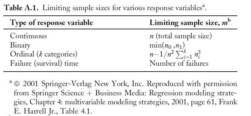
Effective sample size
How to choose predictors
- Subject matter knowledge
- Cost/feasibility of data collection
- Relevance to your research questions
- Potential to be a confounding variable
- Degree of missingness
- Correlation with one or more other variables
- Degree of variability (may want to combine rare categories)
Boostrapping to Evaluate Model stability
How likely are you to end up with the same model if you collect another data set of the same size and apply the same model selection algorithm.
can report bootstrap inclusion frequencies (how often variables are selected in final models)
may want to also report “competitive models” (others that are frequently chosen)
don’t trust a single model unless it is almost always chosen
Can also use the bootstrap to get a more honest measure of fit.
AIC and model-averaging
Rather than choose a best model, another approach is to average predictions among “competitive” models or models with roughly equal “support”.
Steps:
- Start by writing down \(K\) biologically plausible models.
- Fit these models and calculate \(AIC\) (trades-offs goodness-of-fit and model complexity)
- Compute model weights, using the \(AIC\) values, reflecting “relative plausibility” of the different models.
\[w_i= \frac{\exp(-\Delta AIC_i)}{\sum_{k=1}^K\exp(-\Delta AIC_k)}\]
where \(\Delta AIC_i\) = \(min_k(AIC_k) - AIC_i\) (difference in AIC between the “best” model and model \(i\))
- Calculate weighted predictions and SEs that account for model uncertainty.
Model Averaging
Use \(AIC\) weights to calculate a weighted average prediction:
\[\hat{\theta}_{avg}=\sum_{k=1}^K w_k\hat{\theta}_k\]
Calculate a standard error that accounts for model uncertainty and sampling uncertainty:
\[\widehat{SE}_{avg} = \sum_{k=1}^K w_k\sqrt{SE^2(\hat{\theta}_k)+ (\hat{\theta}_k-\hat{\theta}_{avg})^2}\]
Typically, 95% CIs are formed using \(\hat{\theta}_{avg} \pm 1.96\widehat{SE}_{avg}\), assuming that \(\hat{\theta}_{avg}\) is normally distributed.
References
Burnham, Kenneth P., and David R. Anderson. Model selection and multimodel inference: a practical information-theoretic approach. Springer, 2002.
For a counter-point, see (optional reading on Canvas):
Cade, B. S. (2015). Model averaging and muddled multimodel inferences. Ecology, 96(9), 2370-2382.