The Role of Probability in Regression Models
FW8051 Statistics for Ecologists
Learning Objectives
Understand the role of random variables and common statistical distributions in formulating modern statistical regression models.
- Will need to know something about other statistical distributions
- Will need to have an understanding of basic probability theory
- Probability rules and random variables
- Probability mass and probability density functions
- Expected Value and Variance
- How to work with probability distributions in R…
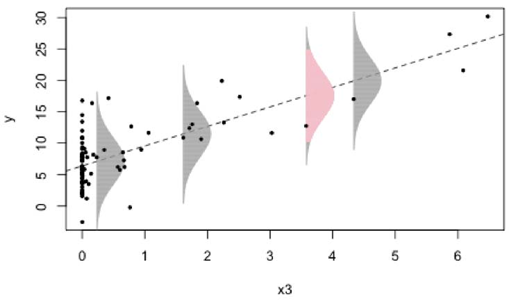
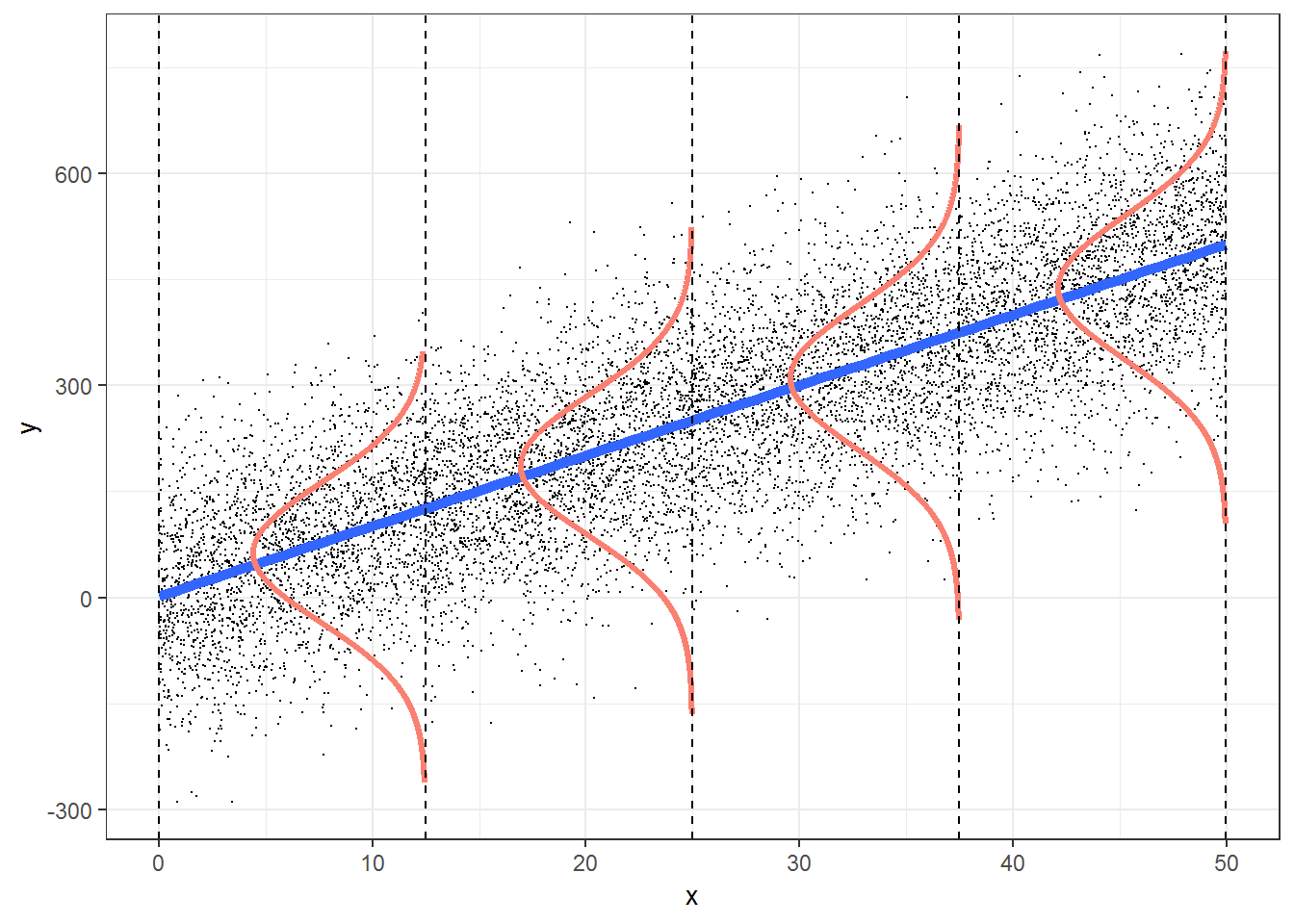
Linear Regression \(y_i = \underbrace{\beta_0 + x_i\beta_1}_\text{Signal} + \underbrace{\epsilon_i}_\text{noise}\)
- Estimated errors, \(\hat{\epsilon}_i\) given by vertical distance between points and the line1
- Find the line that minimizes the errors
Linear Regression
\[Y_i \sim N(\mu_i, \sigma^2)\] \[\mu_i = \beta_0+\beta_1X_i\]
Instead of errors, think about the normal distribution as a data-generating mechanism:
- The line gives the expected (average) value, \(\mu_i\)
- Normal curve describes the variability about this expected value.
Generalizing to other probability distributions
Replace the normal distribution as the data-generating mechanism with another probability distribution, but which one?
It depends on the characteristics of the data
- Does the response variable take on a continuous range of values, only integers, or is it a categorical variable taking on only 1 of 2 values?
Before we learn about different distributions, we need to know a bit more about how we measure probabilities!
Random variables
A random variable is a mapping that takes us from random events to random numbers.
Discrete Random Variables can take on a finite (or countably infinite1) set of possible values.
- Number of birds seen on a plot {0, 1, 2, …}
- Whether or not a moose calf survives its first year {yes, no} \(\rightarrow\) {0, 1}
Continuous Random variables take on random values within some interval.
- T = the age at which a randomly selected white-tailed deer dies (0, \(\infty\))
- W = Mercury level (ppm) in a randomly chosen walleye from Lake Mille Lacs [0, \(\infty\))
- (x, y) such that x,y falls within the continental US
Discrete random variables
Probability Mass Function
A probability mass function, \(p(x)\), assigns a probability to each value that a discrete random variable, \(X\), can take on.
- Flip a coin twice, with the following possible random events: {HH, TH, HT, TT}
- Let \(X\) be a discrete random variable that counts the number of heads (0, 1, or 2).
Probability mass function:
| x | p(x) |
| 0 | 1/4 |
| 1 | 1/2 |
| 2 | 1/4 |
Note: for any probability mass function \(\sum p(x) = 1\)
Bernoulli Distribution
Many categorical response variables can take on only one of two values (dead or alive, migrated or not, etc.)
A Bernoulli random variable, \(X\), maps the two possibilities to the numbers {0, 1} with probabilities \(1-p\) and \(p\), respectively.
| x | p(x) |
| 0 | 1-p |
| 1 | p |
\[X \sim Bernoulli(p)\]
Probability mass function:
\[p(x) = P(X = x) = p^x(1-p)^{1-x}\]
Mean of a Discrete Random Variable
The mean for a discrete random variable with probability function, p(x), is given by:
\[E[X] = \sum_{x} xp(x)\]
\[X \sim Bernoulli(p)\]
| x | p(x) |
| 0 | 1-p |
| 1 | p |
- \(E[X] = \sum\limits_{x\in (0,1)} xp(x) =\) \(0(1-p) + 1p = p\)
Variance and Standard Deviation
The variance for a discrete random variable with probability function, p(x), and mean \(E[x]\) is given by:
\(Var(X) = E(X-E(X))^2 = \sum \limits_{x} (x-E[x])^2p(x) = E[x^2]-(E[x])^2\)
The standard deviation is \(\sigma=\sqrt{Var(x)}\)
\[X \sim Bernoulli(p)\]
| x | p(x) |
| 0 | 1-p |
| 1 | p |
- \(Var[X] = \sum\limits_{x\in (0,1)} (x-E[x])^2p(x)\) \(=(0-p)^2(1-p) + (1-p)^2p = p(1-p)\)
Continuous random variables
Probability Density Function f(x)
\[X \sim N(\mu, \sigma^2)\]
\[f(x) = \frac{1}{\sqrt{2\pi}\sigma}\exp\left(-\frac{(x-\mu)^2}{2\sigma^2}\right)\]
Probabilities are measured in terms of areas under the curve, \(f(x)\):
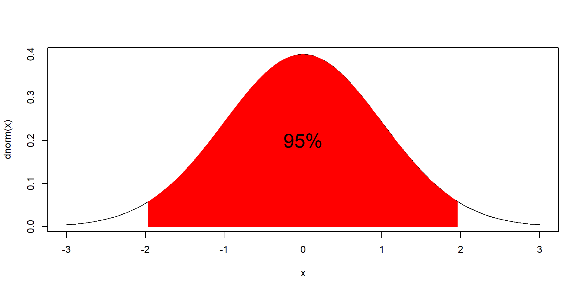
\[P(-1.96 < X < 1.96) = \int_{-1.96}^{1.96} f(x)dx = 0.95\]
- Probability of any point, P\((X = x)\) = 0
- P(a \(\le X \le\) b) = P(a \(< X <\) b)
Cumulative Density Function F(x)
Probability density function, \(f(X)\)
Cumulative distribution function, \(F(X) = P(X \le x)= \int_{-\infty}^{x}f(x)dx\)
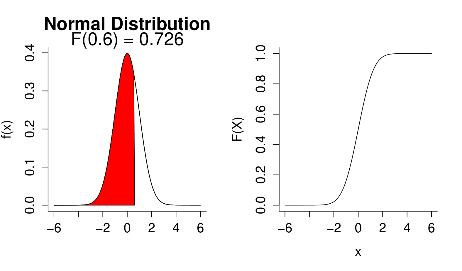
- Unlike probabilities f(x) can be greater than 1
- \(\int f(x)dx = 1\) (area under the curve is one)
- \(F(x)\) goes from 0 to 1
E[X], Var[X], Continuous random variables
Replace sums with integrals!
Mean: \(E[X] = \mu = \int_{-\infty}^{\infty}xf(x)dx\)
Variance: \(Var(X) = \int_{-\infty}^{\infty}(x-E[X])^2f(x)dx\)
Distributions in R
For each probability distribution in R, there are 4 basic probability functions, starting with either - d, p, q, or r:
d is for “density” and returns the value of f(x) - probability density function (continuous distributions) - probability mass function (discrete distributions).
p is for “probability”; returns a value of F(x), cumulative distribution function.
q is for “quantile”; returns a value from the inverse of F(X); also know as the quantile function.
r is for “random”; generates a random value from the given distribution.
Functions in R
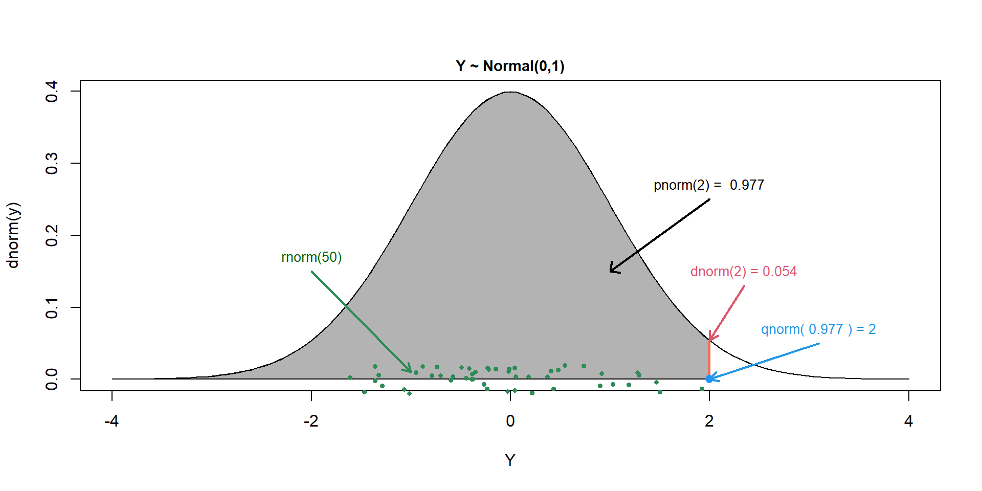
Use this graph, and R help functions if necessary, to complete Exercise 9.1 in the companion book.
Normal Distribution \(X \sim N(\mu, \sigma^2)\)
\[f(x) = \frac{1}{\sqrt{2\pi}\sigma}\exp\left(-\frac{(x-\mu)^2}{2\sigma^2}\right)\]
Parameters:
- \(\mu = E[X]\)
- \(\sigma^2 = Var[X]\)
Characteristics:
- Mean and variance are independent (knowing one tells us nothing about the other)…this is unique!
\(X\) can take on any value (i.e., the range goes from \(-\infty\) to \(\infty\)) …
R normal functions: dnorm, pnorm, qnorm, rnorm.
JAGS: dnorm
Why is the Normal Distribution so Popular
- Central limit theorem (as \(n\) gets large, \(\bar{x}, \sum x\)) become normally distributed
- Model for measurements that are influenced by a large number of factors that act in an additive way
Other notes:
- In JAGS, WinBugs, specified in terms of precision \(\tau = 1/\sigma^2\)
- In R, specified in terms of \(\sigma\) not \(\sigma^2\).
- Often used for priors (Bayesian analysis) to express ignorance (e.g., N(0,100) for regression parameters).
log-normal Distribution: \(X \sim\) Lognormal\((\mu,\sigma)\)
- \(X\) has a log-normal distribution of if \(\log(X) \sim N(\mu, \sigma^2)\)
- \(\mu\) and \(\sigma\) are the mean and variance of log(\(X\)) not \(X\)
- Range: > 0
- R: dlnorm, plnorm, qlnorm, rlnorm with parameters and
- \(E[X] = \exp(\mu+ \sigma^2/2)\)
- \(Var(X)= \exp(2\mu + \sigma^2)(\exp(\sigma^2)-1)\)
- \(Var(X) = kE[X]^2\)
Motivation for log-normal
CLT: if we sum a lot of independent things, then we get a normal distribution.
If we multiply a lot of independent things, we get a log-normal distribution, since:
\[log(X_1X_2\cdots X_n) = log(X_1)+log(X_2)+\ldots log(X_n)\]
Possible examples in biology? Population dynamic models
Lognormal Distribution
Explore briefly in R:
Compare to the expressions for the mean and variance as a function of (\(\mu, \sigma\)):
- \(E[X] = \exp(\mu+ 1/2 \sigma^2)\)
- \(Var(X)= \exp(2\mu + \sigma^2)(\exp(\sigma^2)-1)\)
Bernoulli Distribution:
\[X \sim Bernoulli(p)\]
\[f(x) = P(X = x) = p^X(1-p)^{1-x}\]
- One parameter, \(p\), the probability of ‘success’ = \(P(X=1)\)
- \(0 \le p \le 1\)
- \(E[X] = p\)
- \(Var[X] = p(1-p)\)
- JAGS and WinBugs: dbern
- R has only Binomial distribution (next)
Binomial random variable: \(X \sim\) Binomial\((n,p)\)
A binomial random variable counts the the number of “successes” (any outcome of interest) in a sequence of trials where
- The number of trials, n, is fixed in advance
- The probability of success, p, is the same on each trial
- Successive trials are independent of each other
Formally, a binomial random variable arises from a sum of independent Bernoulli random variables, each with parameter, \(p\):
\[Y = X_1+X_2+\ldots X_n\]
Binomial Probability Function
For a binomial random variable with n trials and probability of success p on each trial, the probability of exactly k successes in the n trials is:
\(P(x = k) ={n \choose k}p^k(1-p)^{n-k}\)
\({n \choose k} = \frac{n!}{k!(n-k)!}\) with \(n!\) = \(n(n-1)(n-2) \cdots (2)1\)
- \(E[X] = np\)
- \(Var(X) = np(1-p)\)
- In R: dbinom, pbinom,qbinom,rbinom
size= \(n\) andprob= \(p\) when using these functions.
Free Throws
Raymond Felton’s free throw percentage during the 2004-2005 season at North Carolina was 70%. If we assume successive attempts are independent, what is the probability that he would hit at least 4 out of 6 free throws in 2005 Championship Game (he hit 5)?

\(P(X \ge 4) = P(X=4) + P(X=5) + P(X=6)\)
\(= {6 \choose 4}0.7^{4}0.3^2 + {6 \choose 5}0.7^{5}0.3^1 + 0.7^{6}\)
Multinomial Distribution
\[X \sim Multinomial(n, p_1, p_2, \ldots, p_k)\]
- Records the number of events falling into each of \(k\) different categories out of \(n\) trials.
- Parameters: \(p_1, p_2, \ldots, p_k\) (associated with each category)
- \(p_k = 1-\sum_{i-1}^{k-1}p_i\)
- Generalizes the binomial to more than 2 (unordered) categories
- R: dmultinom, pmultinom, qmultinom, rmultinom.
- JAGS: dmulti
Multinomial distribution
\(X = (x_1, x_2, \ldots, x_k)\) a multivariate random variable recording the number of events in each category
If \((n_1, n_2, \ldots, n_k)\) is the observed number of events in each category, then:
\(P((x_1, x_2, \ldots, x_k) = (n_1, n_2, \ldots, n_k)) = \frac{n!}{n_1!n_2! \cdots n_k!}p_1^{n_1}p_2^{n_2}\cdots p_k^{n_k}\)
Poisson Distribution: \(N_t \sim Poisson(\lambda)\)
Let \(N_t\) = number of events occurring in a time interval of length \(t\). What is the probability of observing \(k\) events in this interval?
\[P(N_t = k) = \frac{\exp(-\lambda t)(\lambda t)^k}{k!}\]
Events in 2-D space, if events occur at a constant rate, the probability of observing \(k\) events in an area of size \(A\):
\[P(N_A = k) = \frac{\exp(-\lambda A)(\lambda A)^k}{k!}\]
If \(A\) or \(t\) is constant:
\[P(N = k) = \frac{\exp(-\lambda )(\lambda)^k}{k!}\]
Poisson distribution
- Single parameter, \(\lambda\) =
lambda. - \(E[X] = Var(X) = \lambda\)
- R: dpois, ppois, qpois, and rpois.
- JAGS: dpois
Examples:
- Spatial statistics (null model of “complete spatial randomness”“)
- Can be motivated by random event processes with constant rates of occurrence in space or time
Poisson distribution
Suppose a certain region of California experiences about 5 earthquakes a year. Assume occurrences follow a Poisson distribution. What is the probability of 3 earthquakes in a given year?
Geometric Distribution
Number of failures until you get your first success.
\[f(x) = P(X = x) = (1-p)^xp\]
- Parameter = \(p\) (probability of success)
- Range: {0, 1, 2, …}
- \(E[X] = \frac{1}{p} -1\)
- \(Var[X] = \frac{(1-p)}{p^2}\)
- *geom
Negative Binomial: Classic Parameterization
\(X_r\) = Number of failures, \(x\), before you get \(r\) successes; \(X_r \sim\) NegBinom(\(p\))
- Total of \(n = x+r\) trials
- Last trial is a success (\(p\))
- The preceding \(x+r-1\) trials had \(x\) failures (equiv. to a binomial experiment)
\(P(X = x) = {x+r-1 \choose x}p^{r-1}(1-p)^xp\)
or
\(P(X = x) = {x+r-1 \choose x}p^{r}(1-p)^x\)
- \(E[X] = \frac{r(1-p)}{p}\)
- \(Var[X] = \frac{r(1-p)}{p^2}\)
Ecological Parameterization
Express \(p\) in terms of mean, \(\mu\) and \(r\):
\[\mu = \frac{r(1-p)}{p} \Rightarrow p = \frac{r}{\mu+r} \text{ and }\]
\[1-p = \frac{\mu}{\mu+r}\]
Plugging these values in to \(f(x)\) and changing \(r\) to \(\theta\), we get:
\(P(X = x) = {x+\theta-1 \choose x}\left(\frac{\theta}{\mu+\theta}\right)^{\theta}\left(\frac{\mu}{\mu+\theta}\right)^x\)
Then, let \(\theta\) = dispersion parameter take on any positive number (not just integers as in the original parameterization)
Negative Binomial: \(X \sim\) NegBin(\(\mu, \theta\))
\(P(X = x) = {x+\theta-1 \choose x}\left(\frac{\theta}{\mu+\theta}\right)^{\theta}\left(\frac{\mu}{\mu+\theta}\right)^x = \frac{(x+\theta-1)!}{x!(\theta-1)!}\left(\frac{\theta}{\mu+\theta}\right)^{\theta}\left(\frac{\mu}{\mu+\theta}\right)^x\)
- \(E[X] = \mu\)
- \(Var(X) = \mu + \frac{\mu^2}{\theta}\)
- In r: *nbinom, with parameters (
prob= p,size= \(n\)) or (mu= \(\mu\),size= \(\theta\)) - JAGS: dnegbin with parameters (\(p\), \(\theta\))
Overdispersed relative to Poisson (Var(x)/E[x] = 1 + \(\frac{\mu}{\theta}\)) versus 1 for Poisson
Poisson is a limiting case (when \(\theta \rightarrow \infty\))
Negative Binomial
Its appeal for use as a probability generating mechanism in ecology includes the following.
- Allows for non-constant variance typical of count data.
- It often fits zero-inflated data well (and much better than a Poisson distribution).
- It respects the discreteness of the data (no need to transform).
- It can be motivated biologically - e.g.:
If: \(X_i \sim\) Poisson(\(\lambda_i\)), with \(\lambda_i \sim\) Gamma(\(\alpha,\beta\)), then \(X_i\) has a negative binomial distribution.
Continuous Uniform
If observations are equally likely within an interval (A,B):
\[f(x) = \frac{1}{b-a}\]
- Two parameters (a, b)
- Model of ignorance for prior distributions
- \(E[X] = (a+b)/2\)
- \(Var(X) = \sqrt{(b-a)^2/12}\)
- *unif
- JAGS: dunif(lower, upper)
Gamma Distribution: \(X \sim\) Gamma(\(\alpha, \beta\))
\[f(x) = \frac{1}{\Gamma(\alpha)}x^{\alpha-1}\beta^\alpha\exp(-\beta x)\]
- Range 0 to \(\infty\)
- \(\Gamma(\alpha)\) is a generalization of the factorial function (!) that we’ve seen earlier
- \(\alpha\) and \(\beta\) are parameters \(>\) 0.
- \(E[X] = \frac{\alpha}{\beta}\)
- \(Var[X] =\frac{\alpha}{\beta^2}\)
- R: *gamma
Beta Distribution: \(X \sim\) Beta(\(\alpha, \beta\))
\[f(x) = \frac{\Gamma(\alpha+\beta)}{\Gamma(\alpha)\Gamma(\beta)}x^{\alpha-1}(1-x)^{\beta-1}\]
- ranges from 0 to 1.
- \(\alpha\) and \(\beta\) are parameters \(>\) 0.
- \(E[X] = \frac{\alpha}{\alpha+\beta}\)
- \(Var[X] =\frac{\alpha}{(\alpha+\beta)^2(\alpha+\beta+1)}\)
- R: *beta
Exponential: \(X \sim\) Exp(\(\lambda\))
\[f(x) = \lambda \exp(-\lambda x)\]
- Range 0 to \(\infty\)
- \(\lambda > 0\)
- \(E[X] = \frac{1}{\lambda}\)
- \(Var[X] =\frac{1}{\lambda^2}\)
- R: *exp
Distributions
How do we choose an appropriate distribution for our data?
- Presence-absence (0,1) at M sites \(\rightarrow\) Bernoullli/Binomial distribution
- Counts, fixed number of sites/trials/etc \(\rightarrow\) Binomial distribution
- Counts, in a fixed unit of time, area
- Normal distribution if the counts are large
- Poisson distribution: if \(E[Y |X] \approx Var(Y|X)\)
- If \(Var(Y|X) > E(Y|X)\): Negative Binomial, Quasipoisson, Poisson-normal model
- Continuous response variable: normal distribution (usual default)
- gamma (if \(Y\) must be \(> 0\))
- lognormal (if skewed data)
- Time to event: exponential, Weibull
- Cicular data (\(-\pi, \pi\)): von Mises
Other useful information
Note that some can be written in multiple ways:
For example, gamma:
\[f(x) = \frac{1}{\Gamma(\alpha)}x^{\alpha-1}\beta^\alpha \exp(-\beta x)\]
\[f(x) = \frac{1}{\Gamma(\alpha)\beta^\alpha}x^{\alpha-1}\exp(-x/\beta)\]