Probability rules

FW8051 Statistics for Ecologists

Learning objectives

Understand and be able to work with basic rules of probability and probability distributions.

We will need these rules to:

• Understand basics concepts related to Maximum Likelihood and Bayes Theorem; the latter is fundamental to Bayesian statistics.
• Formulate statistical models using different probability distributions.

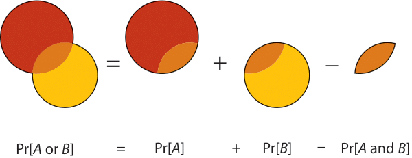
Summary Probability Rules

1. \(P(A \mbox{ and } B) = P(A)P(B \mid A) = P(B)P(A \mid B)\)

2. \(P(A \mbox{ or } B) = P(A) + P(B) - P(A \mbox{ and } B)\)

3. \(P(\mbox{not } A) = 1-P(A)\)

4. \(P(A \mid B) =\frac{P(A \mbox{ and } B)}{P(B)}\) (probability of “A given B”)

[Think-Pair-Share]

Based on recent survey data, 50% of students drink caffeine in the morning, 45% of students drink caffeine in the afternoon, and 37% drink caffeine in the morning and the afternoon. What percent of students who drink caffeine in the morning also drink caffeine in the afternoon?

Want to find: P(A \(|\) M)

= P(A and M)/P(M)

= 0.37/0.50 = 0.74

Caffeine [Think-Pair-Share]

Based on recent survey data, 50% of students drink caffeine in the morning, 45% of students drink caffeine in the afternoon, and 37% drink caffeine in the morning and the afternoon. What percent of students do not drink caffeine in the morning or in the afternoon?

P(not(M or A))

= 1 – P(M or A)

= 1 – [P(M) + P(A) – P(M and A)]

= 1 – [0.50 + 0.45 – 0.37]

= 1 – 0.58 = 0.42

[Think-Pair-Share]

A wildlife biologist surveys 100 different plots, looking for pheasants. Suppose:

• 30% of the plots contain pheasants.

• The biologist has a 60% chance of detecting pheasants when they are present.

On what percentage of the plots should we expect the wildlife biologist to see a pheasant.

P(present and seen) = P(Seen \(|\) present)P(present)

= 0.3 x 0.6 = 0.18

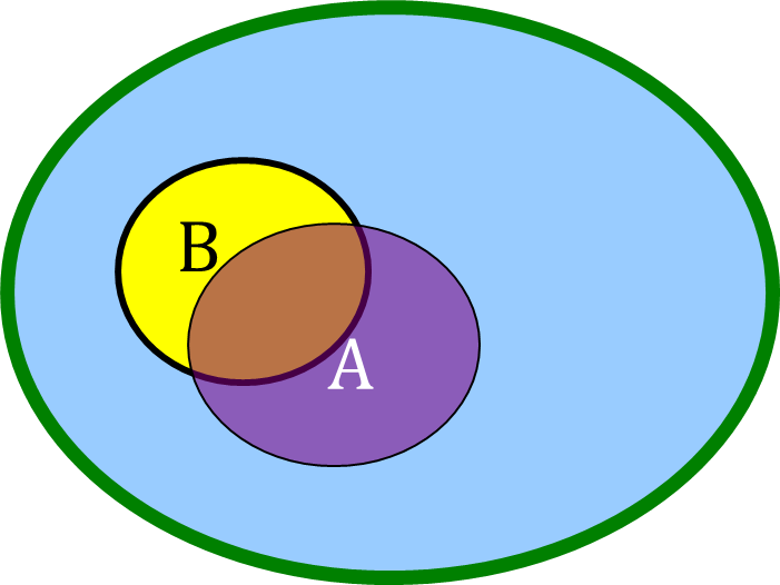
Mutually Exclusive Events

Two events are mutually exclusive if they cannot both be true: P(A and B) = 0.

Sample Space

• Role of a die: {1,2,3,4,5,6}
• Location: {On campus, off campus} (disjoint areas)

What about:

• Mammal and lay eggs: Not mutually exclusive, platypus + four species of echidna

• Teeth and feathers: Yes, mutually exclusive

P(A or B) = P(A) + P(B) for mutually exclusive events.

Independence

Events A and B are independent if \(P(A \mid B) = P(A)\)

Intuitively, knowing that event B happened does not change the probability that event A happened.

If A and B are independent then:

\(P(A \mbox{ and } B) = P(A)P(B \mid A) = P(A)P(B)\)

We have been using this rule to construct Likelihoods!

Summary of Special Cases

If events A and B are mutually exclusive:

• \(P(A \mbox{ or } B) = P(A) + P(B)\)
• \(P(A \mbox{ and } B) = 0\)

If events A and B are independent:

• \(P(A \mid B) = P(A)\)
• \(P(A \mbox{ and } B) = P(A)P(B)\)

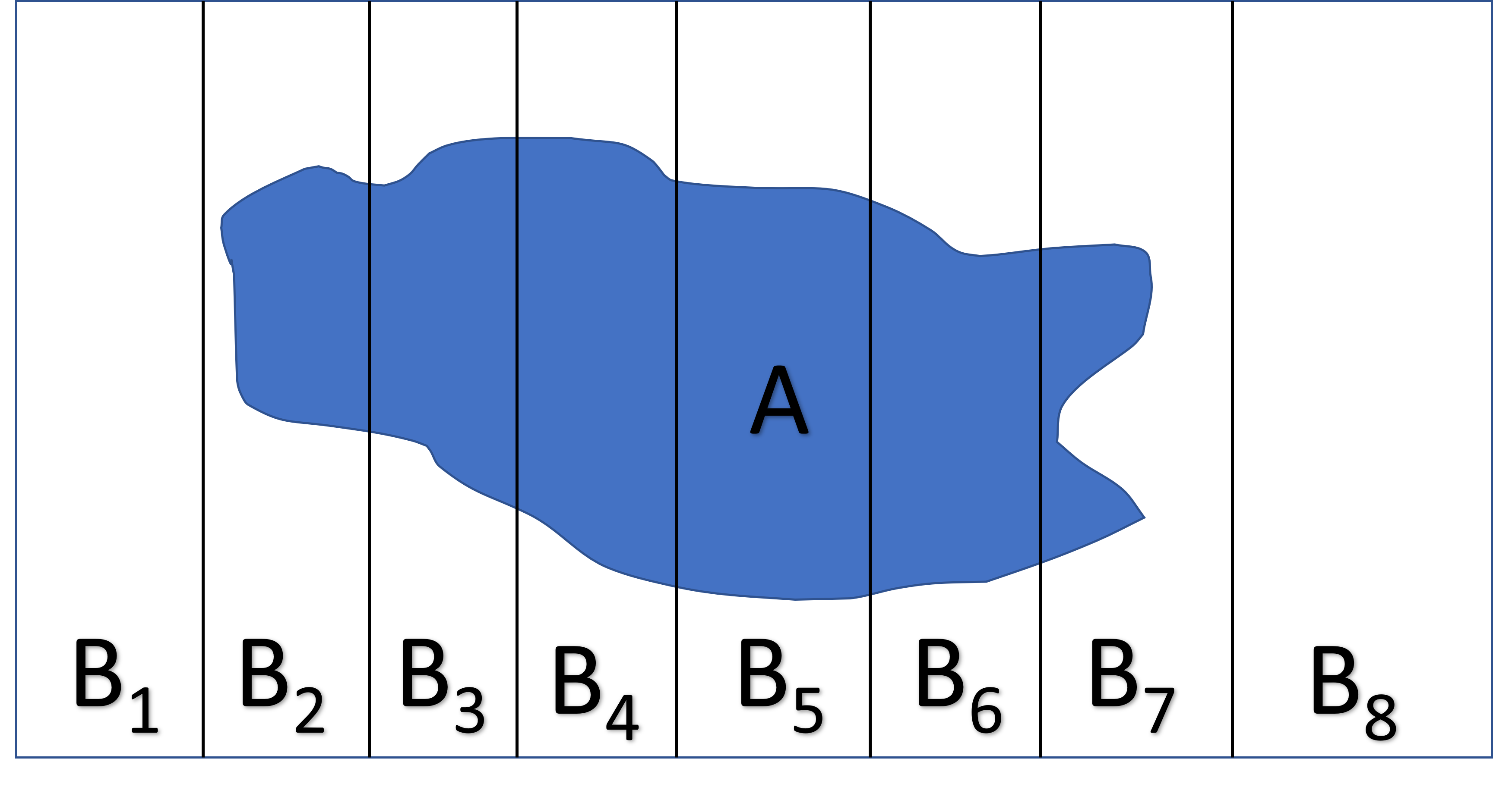
Law of Total Probability

If events \(B_1, B_2, \ldots, B_k\) are mutually exclusive and together make up all possibilities, then:

\(P(A) = \sum_iP(A|B_i)P(B_i)\)

Special Case: \(P(A) = P(A | B)P(B) + P(A | \mbox{not } B)P(\mbox{not } B)\)

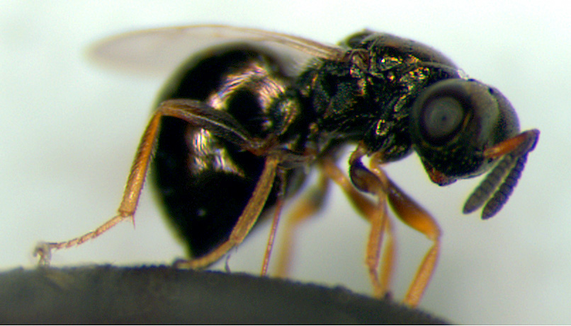
Jewel wasp: from Whitlock and Schluter Example 5.8

Females can manipulate sex of the eggs they lay

• Previously parasitized hosts lay more male eggs
• Other Hosts (not previously parasitized) lay more female eggs

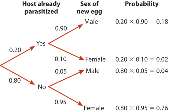
Jewel Wasp [Exercise]

Suppose:

• When a wasp finds a host, there is a 0.20 probability another wasp has already laid eggs in it
• If the host is unparastized, the female lays a male egg with prob = 0.05 (and female egg with prob = 0.95)
• If the host already has eggs, the female lays a male egg with prob = 0.90 (and female egg with prob = 0.10)

Use the total law of probability to determine the probability(sex of new egg is male). Hint: let A = {male}, B = {previously parasitized, not previously parasitized}

Jewel Wasp

Probability(sex of new egg is male)

= P(male & previously parasitized) + P(male & not previously parasitized)

= P(male | previously parasitized)P(previously parasitized) + P(male | not previously parasitized)*P(not previously parasitized)

= 0.2 x 0.9 + 0.05 x 0.8 = 0.22

Tree Diagram

Bayes Theorem

Let \(\bar{A}\) = not(A)

\(P(A \mid B)\) = \(\frac{P(A \normalsize \mbox{ and } B)}{P(B)}\)

\(= \frac{P(B \mid A)P(A)}{P(B \mbox{ and } A) + P(B \mbox{ and } \bar{A}) }\)

\(= \frac{P(B \mid A)P(A)}{P(B \mid A)P(A) + P(B \mid \bar{A})P(\bar{A}) }\)

The last two expressions can be extended to more than 2 groups using the total law of probability

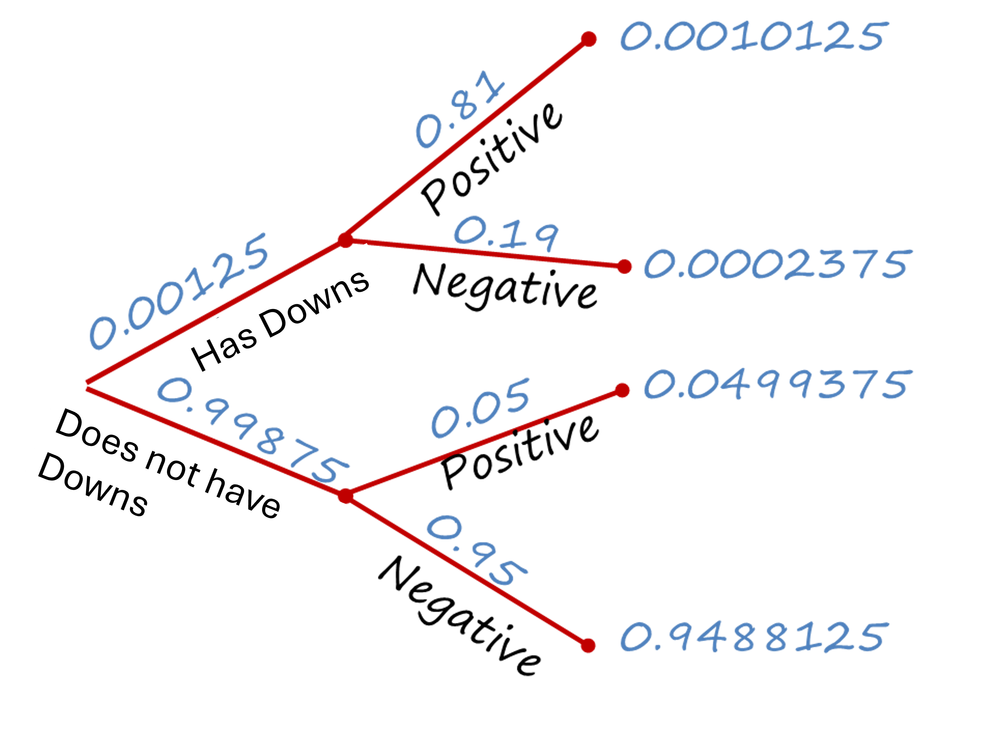
Example: Trisomy 21 or Down Syndrome

Caused by an extra copy of chromosome 21.

• 1 in 800 children have Down Syndrome, i.e., \(P(D) = 1/800 = 0.00125\)
• A multiple-marker screening test can be performed in the second trimester of pregnancy
• False Positive: \(P(+ | \bar{D}) = 0.05\)
• False Negative: \(P(- | D) = 0.19\)

Given that one tests positive, what is the probability that the fetus has Down Syndrome? \(P(D | +)\)

Use Bayes rule: \(= P(A|B) = \frac{P(B \mid A)P(A)}{P(B \mid A)P(A) + P(B \mid \bar{A})P(\bar{A}) }\). It might also help to draw a probability tree.

Probability Tree

\(P(D \mid +) = P(D \mbox{ and } +)/P(+)\)

= 0.0010125/[0.0010125 + 0.0499375] = 0.02

Lets Make A Deal

• 3 doors (2 goats and 1 car)
• Monte knows where the car is, but you don’t
• You pick a door and Monte opens one of the remaining doors holding a goat.
• Should you switch doors?

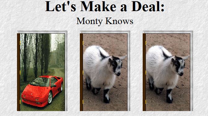
Lets Make A Deal

• 3 doors (2 goats and 1 car)
• Monte knows where the car is, but you don’t
• You pick a door and Monte opens one of the remaining doors holding a goat.
• Should you switch doors?

Answer

4 options, determined by 2 decisions

Step 1:

• You choose the door with the car behind it.
• You choose the door without the car behind it.

Step 2:

• You switch your choice
• You do not switch your choice.

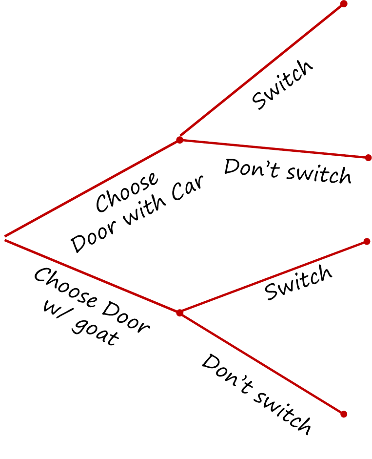
Lets Make A Deal

Probability Tree

P(Win \(|\) Switch) = 0 + 2/3

P(Win \(|\) do not Switch) = 1/3 + 0 = 1/3

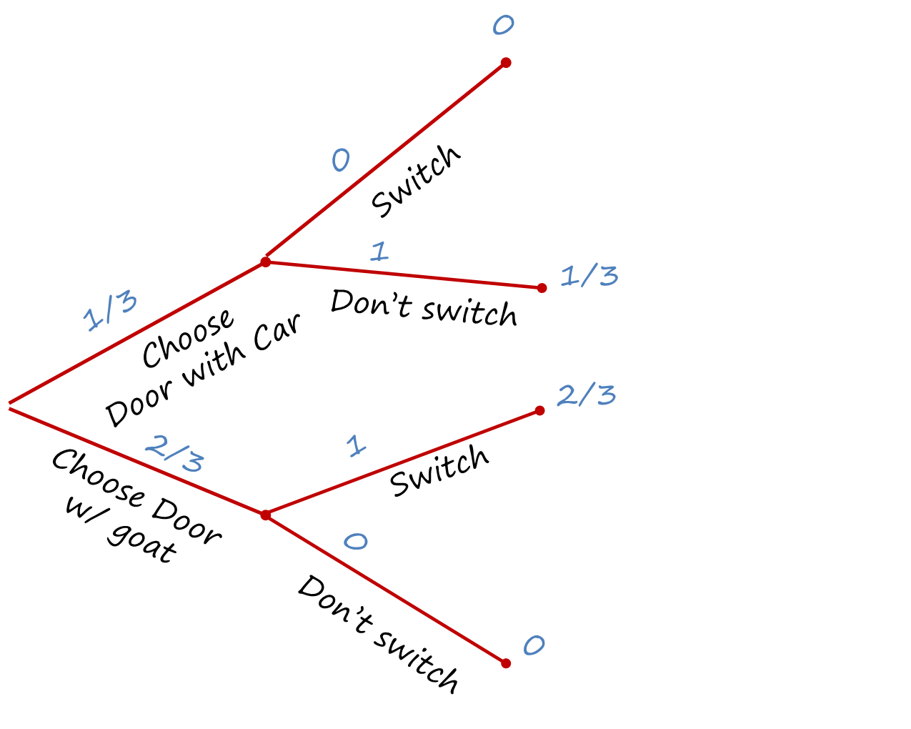
Probability Tree

P(win \(|\) switch) = P(win & switch \(|\) car first)P(car first) + P(win & switch \(|\) goat first)P(goat first) = 0 + 2/3

P(win \(|\) stay put) = P(win & stay put \(|\) car first)P(car first) + P(win & stay put \(|\) goat first)P(goat first) = 1/3 + 0

For some interesting comments on the problem, see this website