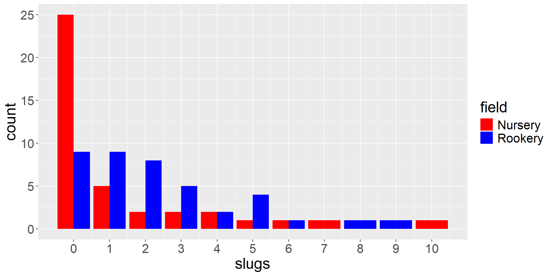
ggplot(slugs, aes(slugs, fill=field))+
  geom_bar(position=position_dodge())+
  theme(text = element_text(size=20))+
   scale_fill_manual(values=c("red", "blue"))+
scale_x_continuous(breaks=seq(0,11,1))Maximum Likelihood
FW8051 Statistics for Ecologists
Learning Objectives
- Understand how to use Maximum Likelihood to estimate parameters in statistical models
- Understand how to create confidence intervals for parameters estimated using Maximum Likelihood
Estimation
We’ve covered a number of statistical distributions, described by a small set of parameters.
- How do we determine appropriate values of the parameters?
- How do we incorporate the effects of covariates?
Methods of estimation:
- Least squares
- Maximum likelihood
- Bayesian methods
Example from Crawley 2002. Statistical Computing and also his The R Book (2007).
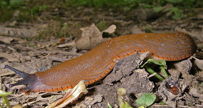
- Counted slugs in 2 fields (rookery, nursery)
- 40 observations in each
Barplot
Hypothesis test
What if we want to use a t-test to test \(H_0: \mu_{rookery} = \mu_{nursery}\)? What do we have to assume?
- The data are normally distributed or sample size is “large enough” for the CLT to apply
Are these assumptions reasonable in light of:
- We have counts (discrete data)
- There were 40 tiles in each of the 2 grasslands (field, nursery)
…maybe (\(n = 30\) is a common rule for CLT to apply)
Alternative Statistical Distributions
Are there other, more appropriate statistical distributions we could use (instead of Gaussian)?
Given that we have count data, we might consider a Poisson or Negative Binomial distribution for the data
We could assume:
- Nursery \(\sim Poisson(\lambda_1)\)
- Rookery \(\sim Poisson(\lambda_2)\)
Test whether \(\lambda_1 = \lambda_2\)
How would we estimate the parameters?
Lets start with the simper case of \(Y_i \sim Poisson(\lambda)\) (ignoring field type)
Maximum Likelihood
Start by writing down a probability statement regarding the data.
Consider the first data point from the Nursery (3 slugs):
\(P(X = 3) = \frac{\exp(-\lambda )(\lambda)^3}{3!}\) if the counts are Poisson distributed
or
\(P(X = 3) = {3+\theta-1 \choose 3}\left(\frac{\theta}{\mu+\theta}\right)^{\theta}\left(\frac{\mu}{\mu+\theta}\right)^3\) if NegBinomial
What about the other observations?
Constructing the Likelihood
Assume the data come from a random sample, and that the points are independent. Then:
\(P(X_1\) =3 & \(X_2 = 0\) & \(\cdots X_{40}=4)\) = \(P(X_1=3)P(X_2=0)\cdots P(X_{40}=4)\)
= \(\frac{\exp(-\lambda )(\lambda)^3}{3!}\frac{\exp(-\lambda )(\lambda)^0}{0!}\cdots \frac{\exp(-\lambda )(\lambda)^4}{4!}\)
More Generally
We obtain a random sample of \(n\) observations from some statistical distribution.
Write down the probability of obtaining the data:
\(P(X_1 =x_1, X_2=x_2, \ldots, X_n = x_n)\) = \(P(X_1=x_1)P(X_2=x_2)\cdots P(X_n=x_n) = \prod_{i=1}^n P(X_i = x_i)\)
For the Poisson distribution:
\[=\frac{\exp(-\lambda )(\lambda)^{x_1}}{x_1!}\frac{\exp(-\lambda)(\lambda)^{x_2}}{x_2!}\cdots \frac{\exp(-\lambda )(\lambda)^{x_n}}{x_n!}\]
\[=\frac{\exp(-n\lambda)(\lambda)^{\sum_{i=1}^nx_i}}{x_1!x_2!\cdots x_n!}\]
This gives us the Likelihood of the data!
Likelihood
For discrete distributions, the likelihood gives us the probability of obtaining the observed data for a particular set of parameters (in this case, \(\lambda\)).
\[P(data; \lambda) = \frac{\exp(-n\lambda)(\lambda)^{\sum_{i=1}^nx_i}}{x_1!x_2!\cdots x_n!} = L(\lambda; data)\]
P(data; parameter):
- Views the data as random, the parameter as fixed.
Likelihood(parameters; data):
- Conditions on the data and considers probability as a function of the parameter.
The maximum likelihood estimate is the value of the parameter, \(\lambda\), that maximizes the likelihood (makes the the observed data most likely)
Maximum Likelihood
The maximum likelihood estimate is the value of the parameter, \(\lambda\), that (i.e., maximizes the likelihood)
\[L(\lambda; x_1, x_2, \ldots, x_n) = \prod_{i=1}^n\frac{\lambda^{x_i}\exp(-\lambda)}{x_i!}\]
How can we find the value of \(\lambda\) that maximizes \(L(\lambda; x_1, x_2, \ldots, x_n)\)?
Calculus (take derivatives with respect to \(\lambda\) and set = 0).
Log-likelihood
For practical and theoretical reasons, we usually work with the log-likelihood (maximizing the log-likelihood is equivalent to maximizing the likelihood)
\[logL(\lambda; x_1, x_2, \ldots, x_n)= log(L(\lambda; x_1, x_2, \ldots, x_n)) = \log(\prod_{i=1}^n P(X_i = x_i))\]
\(= \sum_{i=1}^n log(P(X_i = x_i))\)
For the Poisson model:
\(logL(\lambda; x_1, x_2, \ldots, x_n) = -n\lambda +\log(\lambda)\sum_{i=1}^n X_i - \sum_{i=1}^n \log(x_i!)\)
To maximize, take derivatives and set the expression = 0, giving: …
\[-n + \frac{\sum_{i=1}^n X_i}{\lambda} = 0\]
\[\Rightarrow \hat{\lambda}=\sum_{i=1}^n \frac{X_i}{n}\]
Some notes
To verify that \(\hat{\lambda}\) maximizes (rather than minimizes) \(logL(\lambda| x)\):
- Verify that the \(\frac{\partial^2 logL(\lambda; x)}{\partial \lambda^2}\) evaluated at \(\lambda = \hat{\lambda} =\bar{x} < 0\)
Note: If \(X \sim\) Poisson(\(\lambda\)), \(E[X] = \lambda\)
- It makes sense to estimate \(\lambda\) by the sample mean!
Some constants, e.g., \(\sum_{i=1}^n \log(x_i!)\) do not matter when maximizing the likelihood
- Statistical software may drop/ignore these
- Can matter when comparing models for different probability distributions using AIC
Finding the “best” value of \(\lambda\)
What if we do not remember calculus? How can we find the value of \(\lambda\) that maximizes:
\[L(\lambda; x_1, x_2, \ldots, x_n) = \prod_{i=1}^n\frac{\lambda^{x_i}\exp(-\lambda)}{x_i!}\]
Graph this expression for different values of \(\lambda\)
[Excel in-class exercise]
Finding the “best” values for \(\lambda_1\) and \(\lambda_2\)
What if we had a function of more than 1 parameter? How could we numerically find the value of \(\lambda\) that maximizes:
\[L(\lambda_1, \lambda_2; x_1, x_2, \ldots, x_n) = \prod_{i=1}^{n_{field}}\frac{\lambda_1^{x_i}\exp(-\lambda_{1})}{x_i!} \prod_{j=1}^{n_{rookery}}\frac{\lambda_2^{x_j}\exp(-\lambda_{2})}{x_j!}\]
Use solver in Excel or optim (or glm) in R
[In-class exercise R]
Optim?
Tadpole predation: Example 6.3.1.1 from Bolker et al.(2008)1
\[p = \frac{a}{1+ahN}\]
\[k \sim Binomial(p,N)\]
- \(N\) = number of tadpoles in a tank
- \(k\) = number eaten by predators
We will come back to this or a similar example (in this section and later after introducing Bayesian methods).
Properties of Maximum Likelihood Estimators
\(\hat{\theta}\) = maximum likelihood estimate of \(\theta\).
For large \(n\) (asymptotically):
- Maximum likelihood estimators are unbiased1
- Have minimum variance among estimators
- Will be normally distributed: \(\hat{\theta} \sim N(\theta, I^{-1}(\theta))\)
\(I(\theta)\) is called the Information matrix. Note, it will be a 1 x 1 matrix (or scaler) when estimating a single parameter.
Information Matrix \(I(\theta)\)
Observed information = \(-\frac{\partial^2 logL(\theta)}{\partial \theta^2}\) evaluated at \(\theta = \hat{\theta}\)
Expected information = \(E\left(-\frac{\partial^2 logL(\theta)}{\partial \theta^2}\right)\) evaluated at \(\theta = \hat{\theta}\)
In general, the matrix of second derivatives of a function is called the Hessian.
- \(\left[\frac{\partial^2 logL(\theta)}{\partial \theta^2}\right]\) is the Hessian for \(logL(\theta)\)
- \(\left[-\frac{\partial^2 logL(\theta)}{\partial \theta^2}\right]\) is the Hessian for \(-logL(\theta)\)
Hessian
Consider estimating \(\mu\) and \(\theta\) of the negative binomial distribution by minimizing -\(logL(\mu, \theta)\) (equivalent to maximizing \(logL(\mu, \theta)\).
The Hessian will be given by:
Hessian = \(\begin{bmatrix} -\frac{\partial^2 logL(\mu, \theta)}{\partial \mu^2} & -\frac{\partial^2 logL(\mu, \theta)}{\partial \mu \partial \theta}\\ -\frac{\partial^2 logL(\mu, \theta)}{\partial \mu \partial \theta} & -\frac{\partial^2 logL(\mu, \theta)}{\partial \theta^2}\\ \end{bmatrix}\)
- Used by most optimization routines to find the value of \(\theta\) that minimizes the \(-logL(\theta)\) (we get for “free” when using
optim)
- Inverse of observed information matrix is usually what is reported as \(var(\hat{\theta})\) by statistical software
- We can calculate the involves in R using
solve(object$hessian)
Hessian
The Hessian(\(\theta\)) = \(\left[\frac{\partial^2 logL(\theta)}{\partial \theta^2}\right]\) describes curvature in the log-likelihood curve (surface).
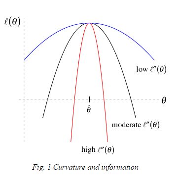
If \(\left[\frac{\partial^2 logL(\theta)}{\partial \theta^2}\right]\) is close to 0:
- The likelihood surface is flat
- LogL is similar across a range of parameter values
Leads to larger confidence intervals since:
- \(I(\theta) = \left[\frac{-\partial^2 logL(\theta)}{\partial \theta^2}\right]\)
- \(\widehat{var}(\hat{\theta}) = I^{-1}(\theta)\)
Application: Growth of black bears
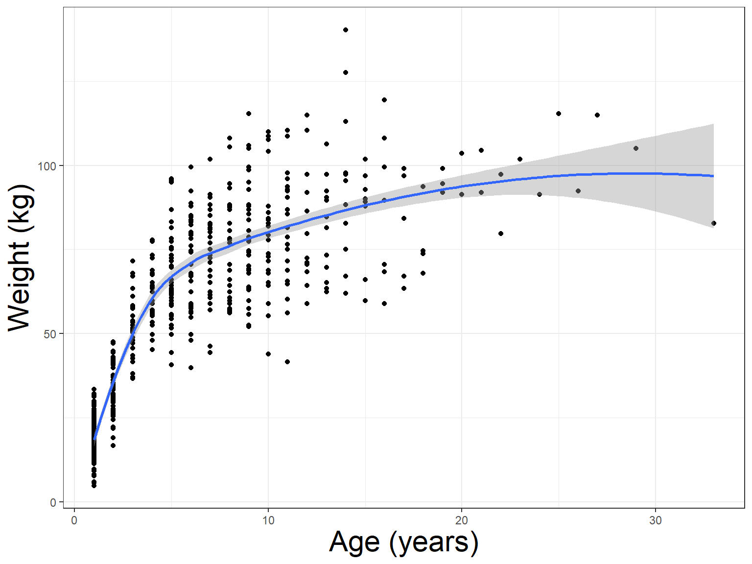
\[Weight_i \sim N(\mu_i, \sigma^2_i)\] \[\mu_i = L_{\infty}(1-e^{-K(Age_i-t_0)})\] \[\sigma^2_i = \sigma^2|\mu_i|^{2\theta}\] [Uing 10-Maximum-Likelihood.R]
Likelihood Ratio Test
A likelihood ratio test can be used to test nested models with:
- The same probability generating mechanism (i.e., same statistical distribution)
- All of the same parameters, except that in one model some parameters are set to specific values (typically 0)
Slug data example:
Full model:
- \(Y_i |\) Nursery \(\sim Poisson(\lambda_1)\)
- \(Y_i |\) Rookery \(\sim Poisson(\lambda_2)\)
Reduced model:
- \(Y_i \sim Poisson(\lambda)\) (i.e., \(\lambda_2= \lambda_1\))
Likelihood Ratio Test
Test statistic:
\[LR = 2log\left[\frac{L(\lambda_1, \lambda_2 | Y)}{L(\lambda | Y)}\right] = 2[logL(\lambda_1, \lambda_2 | Y)-logL(\lambda | Y)]\]
Null distribution (appropriate when \(n\) is large):
\[LR \sim \chi^2_1\]
and more generally \(\chi^2_p\), where \(p\) is the difference in the number of parameters in the two models (See Section 10.9 in book).
Profile Likelihood CIs
Can “invert” the LR test to get profile likelihood-based confidence intervals. Consider generating a CI for \(\lambda\) under the common \(\lambda\) model.
We could use the likelihood ratio test to evaluate:
\(H_0: \lambda = \lambda_0\) vs. \(H_A: \lambda \ne \lambda_0\) for a range of values, \(\lambda_0\).
Compare:
- Full model (\(\lambda\) = Maximum Likelihood estimate, \(\hat{\lambda}_{MLE}\); 1 parameter).
- Reduced model (\(\lambda = \lambda_0\); no estimated parameters)
\[LR = 2log\left[\frac{L(\hat{\lambda} | Y)}{L(\lambda_0 | Y)}\right] \sim \chi^2_1\]
CI for \(\lambda\): include all values for which we do not reject the null hypothesis
Profile Likelihood Intervals
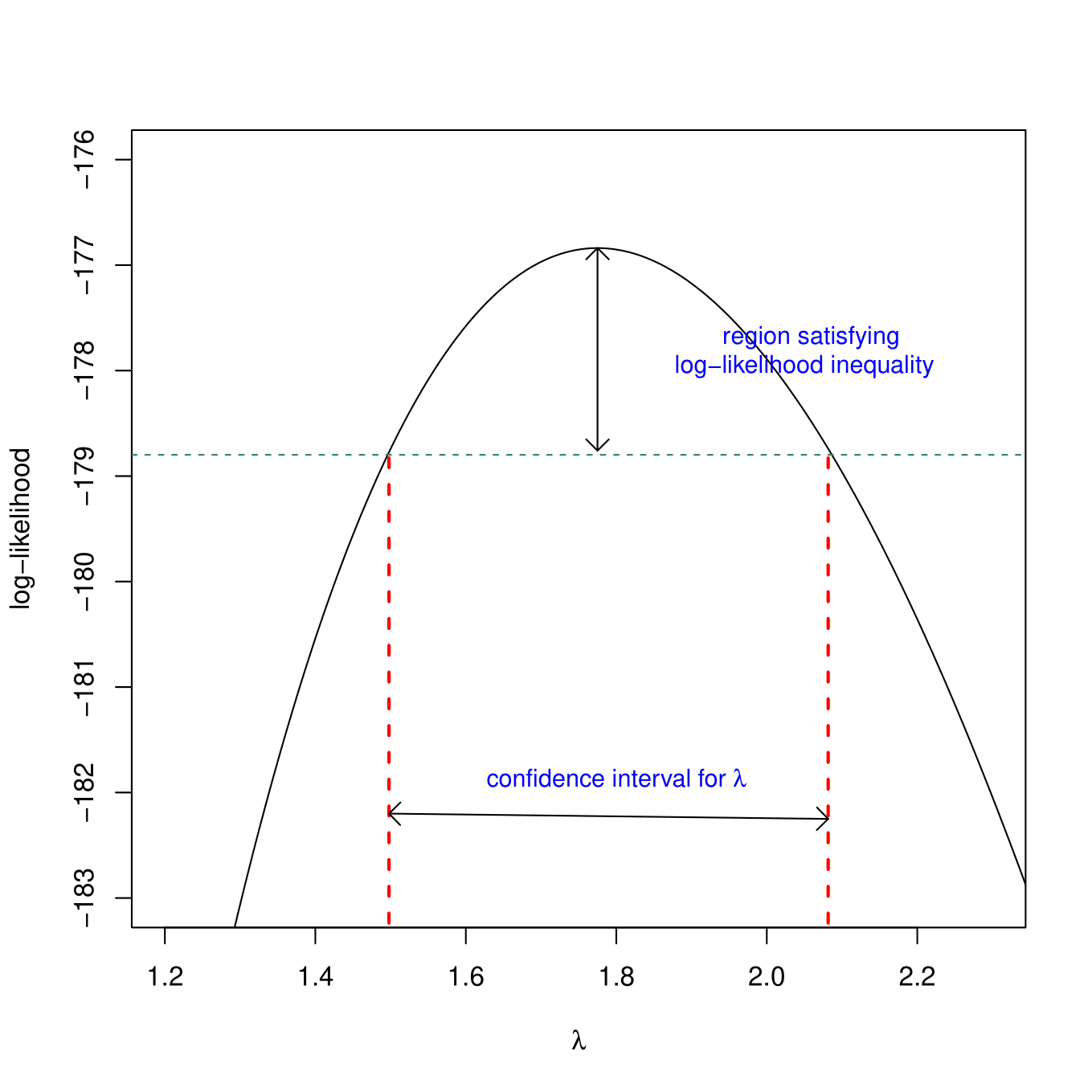
Profile Likelihood Intervals
Can extend to multi-parameter models, e.g., Negative Binomial(\(\mu, \theta\)).
To get a CI for \(\mu\), conduct a series of LR tests for \(H_0: \mu = \mu_0\) vs. \(H_A: \mu \ne \mu_0\)
- Full model: Replace \(\mu\) and \(\theta\) with their Maximum Likelihood estimates (2 estimated parameters)
- Reduced model: Fix \(\mu\) at \(\mu_0\) and estimate the value of \(\theta\) that maximizes this constrained likelihood (1 estimated parameter).
Typically more accurate than normal-based CIs (Wald intervals) when \(n\) is small, but can be computationally heavy to compute.
See Chapter 6 in Bolker’s book (listed in Readings section on Canvas).
Least Squares and MLE
For Normally distributed data:
\(L(\mu, \sigma^2; y_1, y_2, \ldots, y_n) = \prod_{i=1}^n \frac{1}{\sqrt{2\pi}\sigma}\exp\left(-\frac{(y_i-\mu)^2}{2\sigma^2}\right)\)
With linear regression, we assume \(Y_i \sim N(\beta_0 + x_i\beta_1, \sigma^2)\), so…
\(L(\beta_0, \beta_1, \sigma; x) = \prod_{i=1}^n \frac{1}{\sqrt{2\pi}\sigma}\exp\left(-\frac{(y_i-\beta_0+x_i\beta_1)^2}{2\sigma^2}\right) =\frac{1}{(\sqrt{2\pi}\sigma)^n}\exp\left(-\sum_{i=1}^n\frac{(y_i-\beta_0+x_i\beta_1)^2}{2\sigma^2}\right)\)
\(\Rightarrow logL =-nlog(\sigma) - \frac{n}{2}log(2\pi) -\sum_{i=1}^n\frac{(y_i-\beta_0+x_i\beta_1)^2}{2\sigma^2}\)
\(\Rightarrow\) maximizing logL \(\Rightarrow\) minimizing \(\sum_{i=1}^n\frac{(y_i-\beta_0+x_i\beta_1)^2}{2\sigma^2}\)
or, equivalently \(\sum_{i=1}^n(y_i-\beta_0-x_i\beta_1)^2\)