# Estimate and SE
(theta.hat<-59/124)
[1] 0.4758065(se.theta.hat<-sqrt(theta.hat*(1-theta.hat)/124))[1] 0.04484873# Confidence Interval
round(rep(theta.hat,2)+ c(-1.96,1.96)*se.theta.hat,2)[1] 0.39 0.56Understand differences in how probability is defined in Frequentist and Bayesian statistics
Understand how to estimate parameters and their uncertainty using Bayesian methods
Compare Bayesian and Frequentist inference, starting with a simple problem that we can solve analytically.
Goal: make ‘good’ decisions with high probability (across potential repeated experiments)
Still want to make ‘good’ decisions with high probability (across potential repeated experiments)…calibrated Bayes!
Frequentist: relative frequency of events
Bayesian: belief about the system
Lets compare inference from the two methods with a simple example
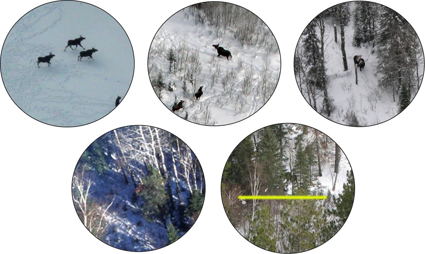
What is the probability, \(p\), that a MNDNR biologist will detect a moose when flying in a helicopter?
Goal: estimate \(p\) and characterize uncertainty wrt \(p\).
Collect data: \(n\) = 124 trials, \(y\) = 59 moose observed …
Make assumptions about the data generating process:
If \(y \sim\) Binomial(n, \(p\)), then:
\(L(p; y) = \frac{n!}{y!(n-y!)}p^{y}(1-p)^{n-y}\)
\(\log(L) = log(\frac{n!}{y!(n-y!)}) + y\log(p) +(n-y)\log(1-p)\)
Maximize \(log[L(p; y)]\) with respect to \(p\) (take derivatives, set equal to 0, and solve) [On Board]:
\(\hat{p} = y/n\)
\(var(\hat{p}) = var(y/n) = var(y)/n^2 = p(1-p)/n\)
We would end up with the same expression if we calculated:
\(I^{-1}(p), \mbox{ where } I(p) = E\left(-\frac{\partial^2 logL(p)}{\partial p^2}\right)\)
For large \(n\), a 95% CI = \(\hat{p} \pm 1.96\sqrt{\frac{\hat{p}(1-\hat{p})}{n}}\)
Where does this come from?
If \(\hat{p} \sim N(p, I^{-1}(p))\), then \(\frac{\hat{p}-p}{\sqrt{var(\hat{p})}} \sim N(0, 1)\)
\(P(-z_{1-\alpha/2} \le \frac{\hat{p}-p}{\sqrt{var(\hat{p})}} \le z_{\alpha/2}) = \alpha\) where \(z\) is a standard normal random variable.
To get a (1-\(\alpha\)) CI, solve the above expression for \(p\).
\[P\left(\hat{p}+ 1.96\sqrt{\frac{\hat{p}(1-\hat{p})}{n}}> p > \hat{p}- 1.96\sqrt{\frac{\hat{p}(1-\hat{p})}{n}}\right) \approx 0.95\]
Calculate the large sample, normal-based confidence interval in R. \(\hat{p} = 59/124 = 0.48\).
x/n and 10,000 95% CIs# 10,000 repeated samples of size 124 and theta = theta.hat
ys<-rbinom(10000,size=124,prob=59/124)
# Calculate 10,000 theta^'s, SE(theta^)'s, CI's
theta.hats<-ys/124
se.theta.hats<-sqrt(theta.hats*(1-theta.hats)/124)
up.CIs<-theta.hats+1.96*se.theta.hats
low.CIs<-theta.hats-1.96*se.theta.hats
# Determine coverage
inCI<-I(low.CIs < 59/124 & up.CIs > 59/124) # true theta is in the interval
sum(inCI)/10000[1] 0.9421In reality, we get 1 data set. We ended up with \(\hat{p}\) = 0.48, with 95% CI = (0.39, 0.56)
How do we interpret this CI?
\(p\) is either in the confidence interval or not! \(P(p \in CI) = 0 \text{ or } 1\)
The procedure we used should result in an interval that contains the true parameter 95% of the time….so,
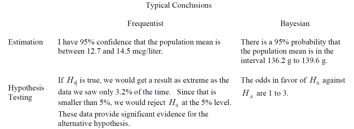
“We are 95% sure that the true parameter is between 0.39 and 0.56.”
How does it differ? What are the steps?
\[p(p | y) = \frac{L(y | p)\pi(p)}{p(y)} = \frac{L(y | p)\pi(p)}{\int L(y | p)\pi(p)dp}\]
The posterior distribution captures our belief about the parameters after having collected data!
\[p(p | y) = \frac{L(y | p)\pi(p)}{p(y)} = \frac{L(y | p)\pi(p)}{\int L(y | p)\pi(p)dp}\]
\(p(y) = \int L(y | p)\pi(p)dp\) is the marginal distribution of \(y\) which requires integrating over \(p\).
In words…
Posterior distribution \(\propto\) Likelihood x prior distribution
Likelihood (from binomial): \(p(y | p) \propto p^{59}(1-p)^{124-59}\)
Prior probability distribution for \(p\)?
[Plot this using curve(dbeta(x, 1, 1), from=0, to=1)]
Use \(\pi(p)\) and \(p(y|p)\) and Bayes Theorem to calculate \(p(p | y)\), the posterior distribution.
\[p(p | y) = \frac{L(y | p)\pi(p)}{p(y)} = \frac{L(y | p)\pi(p)}{\int_{-\infty}^{\infty}L(y | p)\pi(p)d(p)}\]
\[p(p | y) \propto L(y | p)\pi(p)\]
\[p(p |y) \propto p^{59}(1-p)^{124-59}\cdot 1\]
\[p(p |y) \propto p^{60-1}(1-p)^{66-1}\]
This is a beta distribution with parameters (60, 66).
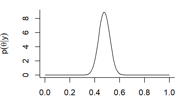
The posterior distribution gives us the probability distribution of the parameter, given the data and our prior beliefs.
Use curve to plot the posterior distribution = Beta(60,66).
Find the endpoints, \(x_1\) and \(x_2\) such that \(P(p \in (x_1,x_2)) = 0.95\).
Use qbeta [remember, \(\alpha = 60, \beta = 66\)]
Same endpoints as Frequentist confidence interval, different interpretation!
Interpretation: \(p\) has a 95% chance of being in the interval.
“Ecologists should be aware that Bayesian methods constitute a radically different way of doing science. Bayesian statistics is not just another tool to be added into ecologists’ repertoire of statistical methods. Instead, Bayesians categorically reject various tenets of statistics and the scientific method that are currently widely accepted in ecology and other sciences. The Bayesian approach has split the statistics world into warring factions (ecologists’ “density independence” vs “density dependence” debates of the 1950s pale by comparison), and it is fair to say that the Bayesian approach is growing rapidly in influence” - Brian Dennis (1996, Ecological Applications, p.1095-1103).
Many do consider Bayesian methods another tool in the toolbox…
We will often fit models using both frequentist and Bayesian statistics (often, with similar answers)!
Dorazio 2016. Population Ecology 58:31-44