MCMC Sampling and JAGS

FW8051 Statistics for Ecologists

Learning objectives

• Gain insights into how MCMC sampling works
• Be able to implement your first Bayesian model in JAGS

Will borrow from…

MCMC

In our moose sighting example, we could determine the posterior distribution using calculus.

In many cases, there will be no closed form solution to:

\[p(\theta | y) = \frac{L(y | \theta)\pi(\theta)}{\int_{-\infty}^{\infty}L(y | \theta)\pi(\theta)}\]

MCMC = Markov Chain Monte Carlo is a way to draw a sequence of random variables that will converge in distribution to \(p(\theta | y)\)

MCMC Sampling

Goal: generate samples that we can use to summarize the posterior distribution, \(p(\theta | y)\)

• Once we have these samples, we can estimate \(\theta\) by the mean (or median) of the samples.
• We can compute credible intervals using quantiles of the samples.

Samplers

There are a variety of MCMC algorithms and samplers. We are going to consider 1 approach to gain somegeneral insights into how these methods work.

Metropolis Algorithm

\[p(\theta | y) = \frac{L(y | \theta)\pi(\theta)}{\int_{-\infty}^{\infty}L(y | \theta)\pi(\theta)}\]

Consider two possible values of \(\theta\) = {\(\theta_1\) and \(\theta_2\)}. Without the denominator, we cannot evaluate \(p(\theta_1 | y)\) or \(p(\theta_2 | y)\).

We can, however, evaluate the relative likelihood of \(\theta_1\) and \(\theta_2\):

\[\text{R } = \frac{p(\theta_2 | y)}{p(\theta_1 | y)} = \frac{L(y | \theta_2)\pi(\theta_2)}{L(y | \theta_1)\pi(\theta_1)}\]

Metropolis Algorithm

1. Initiate the Markov chain with an initial starting value, \(\theta_0\)

2. Generate a new, proposed, value of \(\theta\) from a symmetric distribution centered on \(\theta_0\) (e.g., \(\theta^{\prime}\) = rnorm(\(\theta_0\), mean =0, sd=1)).

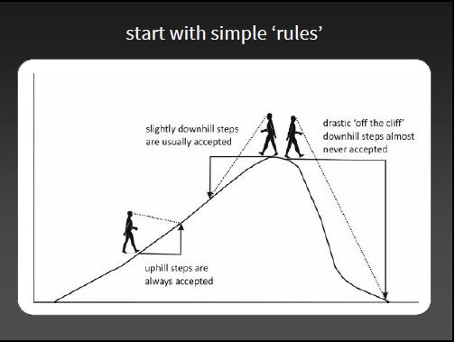
3. Decide whether to accept or reject \(\theta^{\prime}\):

   • If R = \(\frac{p(\theta^{\prime} | y)}{p(\theta_0 | y)} > 1\): Accept and set \(\theta_1 = \theta^{\prime}\)!
     

   • If R \(<1\) accept \(\theta^{\prime}\) with probability = R. Otherwise (i.e., if reject), set \(\theta_1 = \theta_0\)

4. Back to step 2, and …

Continue to sample until:

1. The distribution of \(\theta_1, \theta_2, \ldots, \theta_M\) appears to have reached a steady state (i.e., reached convergence).

2. The MCMC sample, \(\theta_1, \theta_2, \ldots, \theta_M\) is sufficiently large to summarize \(p(\theta | data)\)

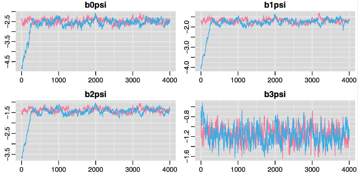
Convergence

There are no foolproof methods for detecting convergence. Some things that we can and will do:

• Run multiple chains (starting in different places) and see if they converge on similar distributions

• Discard the first \(n_{burnin}\) iterations (where the sampler has not yet converged)

• Calculate the Gelman-Rubin Statistic, Rhat = compares variance of between chains to within chains
  • Values near 1 suggest likely convergence
  • Should be less than 1.1 (general rule)

Details

• With Metropolis or Metropolis-Hastings, need to consider how to generate good proposals
• Other samplers may be more efficient (i.e., reach steady state quicker and better explore the distribution of \(p(\theta | data)\))

JAGS will attempt to determine how best to sample once we give it a likelihood and set of prior distributions (one for each parameter).

JAGS

Steps:

• Specify prior distributions and the likelihood of the data.
• Call JAGS from R to generate samples.
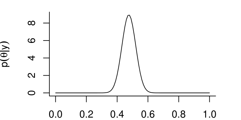
• Evaluate whether or not we think the samples have converged in distribution to \(p(\theta | y)\)
• Use our samples to characterize the posterior distribution, \(p(\theta | data)\)

t-test

Mandible lengths in mm:

• 10 male and 10 female golden jackals
• From British Museum (Manly 1991)

males<-c(120, 107, 110, 116, 114, 111, 113, 117, 114, 112)
females<-c(110, 111, 107, 108, 110, 105, 107, 106, 111, 111)

Do males and females have, on average, different mandible lengths?

\[H_0: \mu_m = \mu_f \text{ versus } H_a: \mu_m \neq \mu_f\]

JAGS

Likelihood:

• \(y_{males} \sim N(\mu_m, \sigma^2)\)
• \(y_{females} \sim N(\mu_f, \sigma^2)\)

Priors:

• \(\mu_m \sim N(100, 0.001)\)
• \(\mu_f \sim N(100, 0.001)\)
• \(\sigma \sim\) Uniform(0,30)

Notes:

• JAGS and WinBugs represent a normal distribution as \(N(\mu, \tau = 1/\sigma^2)\), \(\tau\) is called the precision

• Often best to form priors for \(\sigma\) (requires thinking about SD rather than 1/variance)

Where do these priors come from?

Good question. I tried to make sure:

• the priors were dispersed enough to encompass all the likely values for the parameters

It is a good idea to check whether:

• your posterior looks different from your prior (i.e., if it was “informed by the data”)
• the posterior appears to have been constrained by your prior distribution
• your results change if you use a different prior

JAGS

JAGS/BUGS (hereafter JAGS) code looks just like R code, but with some differences:

• JAGS code is not executed (just defines the model)
• Order does not matter (prior before likelihood, likelihood after prior, etc)

JAGS

There are 6 types of objects

1. Modeled data defined with a \(\sim\) (“distributed as”). For example y \(\sim\) followed by a probability distribution. The variable y here is the response in our regression model.

2. Unmodeled data: objects that are not assigned probability distributions. Examples include predictors, constants, and index variables.

3. Modeled parameters: these are given informative “priors” that themselves depend on parameters called hyperparameters. These are what a frequentist would call random effects. We won’t consider till later in the course.

4. Unmodeled parameters: these are given uninformative priors. [So in truth all parameters are modeled].

5. Derived quantities: these objects are typically defined with the assignment arrow, <-

6. Looping indexes: i, j, etc.

JAGS

Types of objects for JAW example

1. Modeled data = males, females

2. Unmodeled data = nmales, nfemales

3. Modeled parameters (none in this example)

4. Unmodeled parameters = mu.male, mu.female, sigma

5. Derived quantities = tau, mu.diff

6. Looping indexes: i (used twice)

JAGS Tips

Start simple, then build up.

Lots of good tricks and tips in the Appendix of Kery’s Introduction to WinBugs for Ecologists, especially:

Numbers: 2, 3, 4, 9, 11, 12 (use %T% in JAGS), 14, 16, 17, 20, 23,24, 25, 26, 27

Googling error messages is often useful for diagnosing problems.

JAGS

Work with 12-BayesMCMC.R to fit your first model in JAGS