Introduction to Generalized Linear Models
Learning Objectives
Understand the role of random variables and common statistical distributions in formulating modern statistical regression models
Be able to fit appropriate models to count data and binary data (yes/no, presence/absence) in both R and JAGS
Be able to evaluate model goodness-of-fit
Be able to describe a variety of statistical models and their assumptions using equations and text and match parameters in these equations to estimates in computer output.
Outline
- Introduction to generalized linear models
- Models for count data (Poisson and Negative Binomial regression)
- Models for Binary data (logistic regression)
- Models for data with lots of zeros
Linear Regression
Often written in terms of “signal + error”:
\[Y_i = \underbrace{\beta_0 + X_i\beta_1}_\text{Signal} + \underbrace{\epsilon_i}_\text{error}, \mbox{ with}\]
\[\epsilon_i \sim N(0, \sigma^2)\]
Possible because the Normal distribution has separate parameters that describe:
- mean: \(E[Y_i|X_i] = \mu_i = \beta_0 + X_i\beta_1\)
- variance: \(Var[Y_i|X_i] = \sigma^2\)
Remember: for Poisson, Binomial distributions, the variance is a function of the mean.
Linear Regression
\[Y_i|X_i \sim N(\mu_i, \sigma^2)\] \[\mu_i=\beta_0 + \beta_1X_{1,i} + \ldots \beta_pX_{p,i}\]
This description highlights:
- The distribution of \(Y_i\) depends on a set of predictor variables \(X_i\)
- The distribution of the response variable, conditional on predictor variables is Normal
- The mean of the Normal distribution depends on predictor variables (\(X_1\) through \(X_p\)) and regression coefficients (the \(\beta_1\) through \(\beta_p\))
- The variance is constant and given by \(\sigma^2\).
Linear Regression = General Linear Model
Sometimes referred to as: General Linear Model
- t-test (categorical predictor with 2 categories)
- ANOVA (categorical predictor with \(> 2\) categories)
- ANCOVA (continuous and categorical predictor, no interaction so common slope)
- Continuous and categorical variables, with possible interactions
Generalized Linear Models
Generalized linear models further unifies several different regression models:
- General linear model
- Logistic regression
- Poisson regression
Rather elegant general theory developed for exponential family of distributions
Generalized Linear Models (glm)
Systematic component: \(g(\mu_i) = \eta_i = \beta_0 + \beta_1X_1 + \ldots \beta_pX_p\)
Some transformation of the the mean, \(g(\mu_i)\), results in a linear model.
- \(g( )\) is called the link function
- \(\eta_i = \beta_0 + \beta_1X_1 + \ldots \beta_pX_p\) is called the linear predictor.
- \(\mu_i = g^{-1}(\eta_i) = g^{-1}(\beta_0 + \beta_1X_1 + \ldots \beta_pX_p)\)
Random component: \(Y_i|X_i \sim f(y_i|x_i), i=1, \ldots, n\)
- \(f(y_i|x_i)\) is in the exponential family (includes normal, Poisson, binomial, gamma, inverse Gaussian)
- \(f(y_i|x_i)\) describes unmodeled variation about \(\mu_i = E[Y_i|X_i]\)
Generalized Linear Models (glm)
Linear Regression:
- \(f(y_i|x_i) = N(\mu_i, \sigma^2)\)
- \(E[Y_i|X_i]= \mu_i = \beta_0 + \beta_1X_1 + \ldots \beta_pX_p\)
- \(g(\mu_i) =\eta_i = \mu_i\), the identity link
- \(\mu_i = g^{-1}(\eta_i) = \eta_i= \beta_0 + \beta_1X_1 + \ldots \beta_pX_p\)
Poisson regression:
- \(f(y_i|x_i) = Poisson(\lambda_i)\)
- \(E[Y_i|X_i] = \mu_i = \lambda_i\)
- \(g(\mu_i) = \eta_i = log(\lambda_i) = \beta_0 + \beta_1X_1 + \ldots \beta_pX_p\)
- \(\mu_i = g^{-1}(\eta_i) = \exp(\eta_i) = \exp(\beta_0 + \beta_1X_1 + \ldots \beta_pX_p)\)
Other GLMs
Logistic regression:
- \(f(y_i|x_i) =\) Bernoulli\((p_i)\)
- \(E[Y_i|X_i] = p_i\)
- \(g(\mu_i) = \eta_i = logit(p_i) = log(\frac{p_i}{1-p_i}) = \beta_0 + \beta_1X_1 + \ldots \beta_pX_p\)
- \(\mu_i = g^{-1}(\eta_i) = \frac{\exp^{\eta_i}}{1+\exp^{\eta_i}} = \frac{\exp^{\beta_0 + \beta_1X_1 + \ldots \beta_pX_p}}{1+\exp^{\beta_0 + \beta_1X_1 + \ldots \beta_pX_p}}\)
Link functions and sample space
Link functions allow the “structural component” (\(\beta_0 + \beta_1x_1 + \ldots \beta_pX_p\)) to live on \((-\infty, \infty)\) while keeping the \(\mu_i\) consistent with the range of the response variable.
Poisson (counts) = \({0, 1, 2, \ldots, \infty}\)
- \(\log(\lambda_i) = \beta_0 + \beta_1X_1 + \ldots \beta_pX_p\), range = \((-\infty, \infty)\)
- \(\mu_i = \exp(\beta_0 + \beta_1X_1 + \ldots \beta_pX_p)\), range = \([0, \infty]\)
Logistic regression:
- \(log(\frac{p_i}{1-p_i}) = \beta_0 + \beta_1X_1 + \ldots + \beta_pX_p\), range = \((-\infty, \infty)\)
- \(\mu_i = p_i = \frac{\exp(\beta_0 + \beta_1X_1 + \ldots \beta_pX_p)}{1+\exp(\beta_0 + \beta_1X_1 + \ldots \beta_pX_p)}\), range = \((0, 1)\)

Photo by Gary Noon - Flickr, CC BY-SA 2.0, https://commons.wikimedia.org/w/index.php?curid=4077294
- \(X_i\) = amount of grassland cover
- \(Y_i|X_i \sim Poisson(\lambda_i)\)
- \(log(\lambda_i) = \beta_0 + \beta_1X_{i}\)
Because the mean of the Poisson distribution is \(\lambda\):
- \(E[Y_i|X_i] = \lambda_i = \exp(\beta_0 + \beta_1X_i) = \exp(\beta_0)\exp(\beta_1X_i)\)
- The mean number of pheasants increases by a factor of \(\exp(\beta_1)\) as we increase \(X_i\) by 1 unit.
Assumptions
- Poisson Response: The response variable is a count per unit of time or space, described by a Poisson distribution.
- Independence: The observations must be independent of one another.
- Mean=Variance: By definition, the mean of a Poisson random variable must be equal to its variance.
- Linearity: The log of the mean rate, log(\(\lambda\)), must be a linear function of x.
Visually
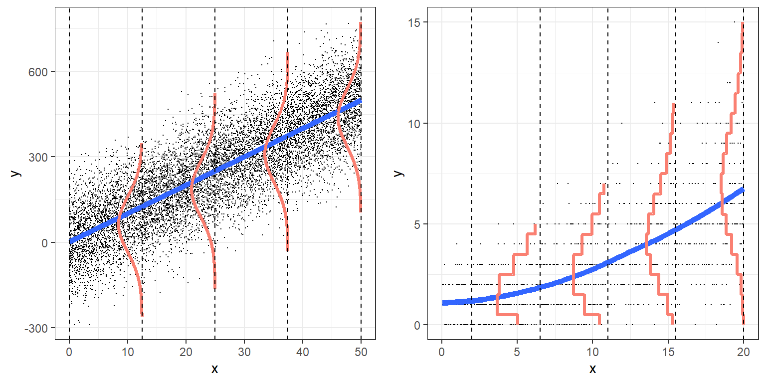
From Broadening Your Statistical Horizons: https://bookdown.org/roback/bookdown-bysh/
Next Steps
- Fit regression models (using ML and Bayesian methods) appropriate for count data
- Poisson regression models
- Negative Binomial regression
- Use an offset to model rates and densities, accounting for variable survey effort
- Use simple tools to assess model fit
- Residuals (deviance and Pearson)
- Goodness-of-fit tests
Next Steps
- Interpret estimated coefficients and describe their uncertainty using confidence and credible intervals
- Use deviances and AIC to compare models.
- Be able to describe statistical models and their assumptions using equations and text and match parameters in these equations to estimates in computer output.