Be able to fit regression models appropriate for count data in R and JAGS
Poisson regression models
Quasi-Poisson (R only)
Negative Binomial regression
Be able to evaluate model fit
Residual plots
Goodness-of-fit tests
Use deviances and AIC to compare models.
Use an offset to model rates and densities, accounting for variable survey effort
Be able to describe statistical models and their assumptions using equations and text and match parameters in these equations to estimates in computer output.
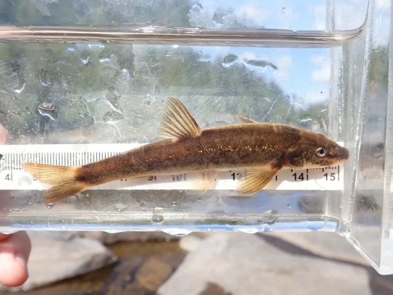
Longnose Dace
longnosedace: number of longnose dace (Rhinichthys cataractae) per 75-meter section of stream.
acreage: area (in acres) drained by the stream.
do2: the dissolved oxygen (in mg/liter).
maxdepth: the maximum depth (in cm) of the 75-meter segment of stream.
no3: nitrate concentration (mg/liter).
so4: sulfate concentration (mg/liter).
temp: the water temperature on the sampling date (in degrees C).
\(\beta_0\) = expected log mean when all predictors are equal to 0
\(\exp(\beta_0)\) = expected mean when all predictors are equal to 0
\(\beta_2\) = 0.226 = expected change in the log mean [i.e., \(\log(\lambda)\)], per unit change in D02, while holding everything else constant.
\(\exp(\beta_2)\) = 1.25 = we expect the mean to increase by a factor of 1.25 for every 1 unit change in D02 (and holding everything else constant)
Inference
Rely on asymptotic Normality for Maximum Likelihood Estimators
\[\hat{\beta} \sim N(\beta, I^{-1}(\theta))\]
# Store coefficients and their standard errorsbeta.hats <-coef(glmPdace)ses <-sqrt(diag(vcov(glmPdace)))round(cbind(beta.hats-1.96*ses, beta.hats+1.96*ses), 3)
\(logL(\hat{\theta}_s | y)\) = log-likelihood for a “saturated” model (one with a parameter for each observation).
\(logL(\hat{\theta}_0 | y)\) = log-likelihood for our model of interest evaluated at the MLEs (\(\hat{\theta}_0\))
Null deviance = residual deviance for a model that only contains an intercept
It may be helpful to think of the null deviance and residual deviance as maximum likelihood equivalents to total and residual sums of squares, respectively.
Deviance
There is no \(R^2\) for generalized linear models, but sometimes see % deviance explained (pseudo \(R^2\)):
Poisson is a limiting case (when \(\theta \rightarrow \infty\))
Negative Binomial Models in R
Can fit negative binomial models in R using the glm.nb function in the MASS library
glm.nb(y ~ x, data=)
Lets do this and inspect goodness of fit!
Model comparisons
For large samples, the difference in deviances for nested models should be \(\sim \chi^2\) with df = difference in number of parameters between the two models.
\[D_2-D_1 \sim \chi^2_{df}\]
Can use drop1(model, test="Chi") (equivalent to a likelihood ratio test) or Anova in car package
Can use forward, backwards, stepwise selection (with the same dangers/caveats related to overfitting); see stepAIC in MASS library (for backwards selection)
AIC
AIC = -2 x \(logL(\hat{\theta} | y)\) + 2 x number of parameters
measure of “fit” with “penalty” for model complexity
the larger log-likelihood, the smaller AIC
for similar likelihoods, AIC will be smaller for simpler models
\(\rightarrow\) smaller AIC is better
Can use to compare nested and non-nested models.
Not always appropriate for certain types of models (problematic if you have latent variables, e.g., mixture models)
Negative Binomial in JAGS
JAGS: dnegbin specified in terms of parameters (\(p\), \(\theta\))
We will specify the model in terms of \(\mu\) and \(\theta\), then solve for \(p\):
\(\log(\mbox{Time}_i)\) is called an offset and can be modeled using:
glm(y ~ x + offset(log(time)), data= , family = poisson())
An offset is an explanatory variable with a regression coefficient fixed at 1.
See PoissonOffsetTemplate.R and PoissonOffset.R (in the Generalized linear models folder) for an exercise fitting a Poisson model with an offset.
DIC
Martyn Plummer (creator of JAGS):
DIC [like AIC] is (an approximation to) a theoretical out-of-sample predictive error.
“The deviance information criterion (DIC) is widely used for Bayesian model comparison, despite the lack of a clear theoretical foundation….valid only when the effective number of parameters in the model is much smaller than the number of independent observations. In disease mapping, a typical application of DIC, this assumption does not hold and DIC under-penalizes more complex models. Another deviance-based loss function, derived from the same decision-theoretic framework, is applied to mixture models, which have previously been considered an unsuitable application for DIC.”
DIC
Andrew Gelman: “I don’t really ever know what to make of DIC. On one hand, it seems sensible…On the other hand, I don’t really have any idea what I would do with DIC in any real example. In our book we included an example of DIC–people use it and we don’t have any great alternatives–but I had to be pretty careful that the example made sense. Unlike the usual setting where we use a method and that gives us insight into a problem, here we used our insight into the problem to make sure that in this particular case the method gave a reasonable answer.”
Model comparisons
There are other potential options out there (e.g., WIC, cross-validation estimates of predictive error, etc)
Hooten, Mevin B, and N Thompson Hobbs. 2015. “A Guide to Bayesian Model Selection for Ecologists.” Ecological Monographs 85 (1): 3–28.