Logistic regression models for binary data
FW8051 Statistics for Ecologists
Learning Objectives
Be able to formulate, fit, and interpret logistic regression models appropriate for binary data using R and JAGS
Be able to compare models and evaluate model fit
Be able to visualize models using effect plots
Be able to describe statistical models and their assumptions using equations and text and match parameters in these equations to estimates in computer output
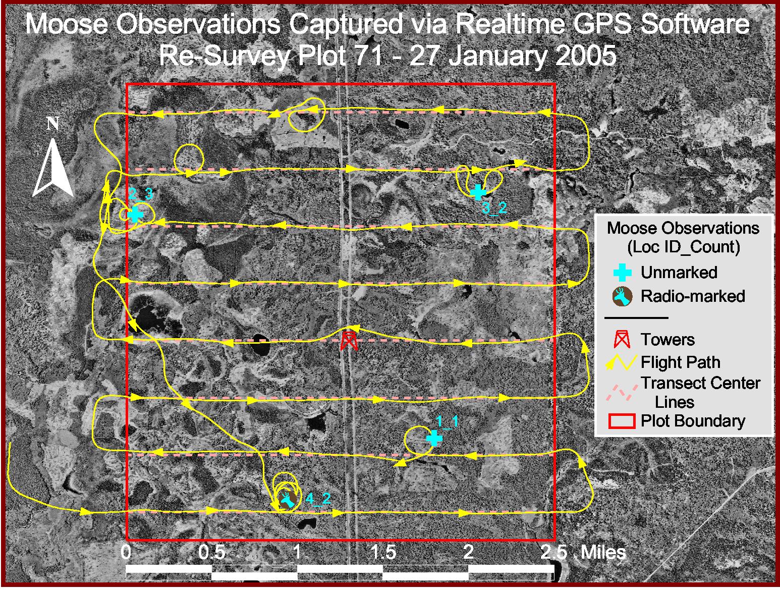
Sightability Surveys: Minnesota Moose
124 trials, 2005-2007
\(n_0\) = 65 missed groups\(n_1\) = 59 observed groups
Binary observations, \(Y_i = 0 \mbox{ (missed) or } 1 \mbox{ (seen)}\) .
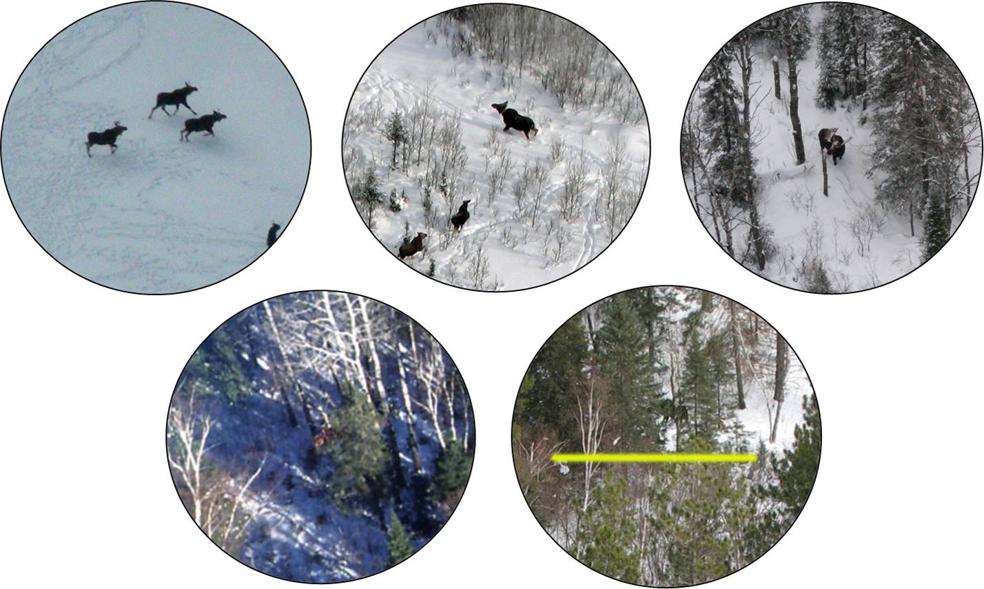
Covariates thought to influence detection.
Covariates {f.90}
Visual obstruction
Survey year (may be due to different observers)
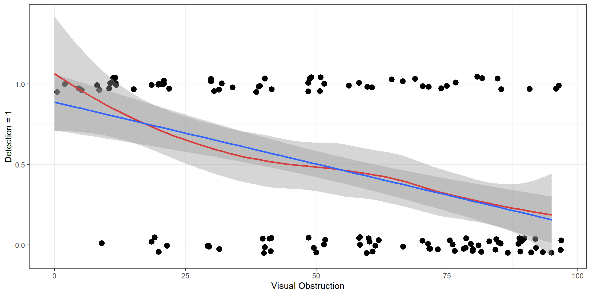
Visual Obstruction
ggplot (exp.m, aes (voc,observed))+ theme_bw ()+ geom_point (position = position_jitter (w = 2 , h = 0.05 ), size= 3 ) + geom_smooth (colour= "red" ) + geom_smooth (method= "lm" )+ xlab ("Visual Obstruction" ) + ylab ("Detection = 1" )
lm could lead to predictions where \(p_i \ge 1\) and \(p_i \le 0\) lm assumes constant variance rather than \(var(p_i) = p_i(1-p_i)\)
Logistic regression
Model for binary (0/1) data or binomial data (number of 1’s out of \(n\) trials).
\[Y_i | X_i \sim Bernoulli(p_i)\]
\[logit(p_i) = log\left(\frac{p_i}{1-p_i}\right) = \beta_0 + \beta_1 X_{1,i}+ \ldots \beta_p X_{p,i}\]
Random component = Bernoulli or binomial distribution
Systematic component: logit(\(p_i\) ) or log(odds) = linear combination of predictors
Remember, for binary data, \(E[Y_i|X_i] = p_i\) , \(Var[Y_i|X_i] = p_i(1-p_i)\)
\(\Rightarrow p_i = \frac{\exp(\beta_0 + \beta_1 X_{1,i}+ \ldots \beta_p X_{p,i})}{1+\exp(\beta_0 + \beta_1 X_{1,i}+ \ldots \beta_p X_{p,i})}\)
(can use plogis function in R)
Logistic regression
\[Y_i | X_i \sim Bernoulli(p_i)\]
\[logit(p_i) = log\left(\frac{p_i}{1-p_i}\right) = \beta_0 + \beta_1 X_{1,i}+ \ldots \beta_p X_{p,i}\]
\(\frac{p}{1-p}\) is referred to as the odds .
The link function, \(\log \Big(\frac{p}{1-p}\Big)\) , is referred to as logit .
Thus, we can describe our model in the following ways:
We are modeling \(\log \Big(\frac{p}{1-p}\Big)\) as a linear function of \(X_1, \dots, X_p\) .
We are modeling the logit of \(p\) as a linear function of \(X_1, \dots, X_p\) .
We are modeling the log odds of \(p\) as a linear function of \(X_1, \dots, X_p\) .
Odds = \(\frac{p}{1-p}\)
If the probability of winning a bet is = 2/3, what are the odds of winning?
odds = \(\frac{p}{1-p}\) = (2/3 \(\div\) 1/3) = 2 (or “2 to 1”).
Relationship between probability (p), odds, and log odds.
log odds \(= \log\Big(\frac{p}{1-p}\Big)\)
-6.907
-1.386
0.0
1.386
6.907
odds \(= \frac{p}{1-p}\)
0.001
0.250
1.0
4.000
999.000
p
0.001
0.200
0.5
0.800
0.999
Odds can vary between 0 and \(\infty\) , so log(odds) can live on \(-\infty\) to \(\infty\) .
Odds Ratios: \(\exp(\beta)\)
Consider a regression coefficient for a categorical variable:
\[logit(p_i) = log(\frac{p_i}{1-p_i}) = \beta_0 + \beta_1I(group=B)_i\]
\(I(group=B)_i\) = 1 if observation \(i\) is from Group B and 0 if Group A
Odds for group B = \(\frac{p_B}{1-p_B} = \exp(\beta_0+\beta_1)\)
Odds for group A = \(\frac{p_A}{1-p_A} = \exp(\beta_0)\)
Consider the ratio of these odds:
\[\frac{\frac{p_B}{1-p_B}}{\frac{p_A}{1-p_A}} = \frac{\exp(\beta_0+\beta_1)}{\exp(\beta_0)} =\frac{e^{\beta_0}e^{\beta_1}}{e^{\beta_0}}= \exp(\beta_1)\]
So, \(\exp(\beta_1)\) gives an odds ratio (or ratio of odds) for Group B relative to group A.
Odds Ratios: \(\exp(\beta)\)
Consider a continuous predictor, \(X\) :
\[logit(p_i) = log(\frac{p_i}{1-p_i}) = \beta_0 + \beta_1X_i\]
\(\beta_1\) gives the change in log odds per unit change in \(X\) .
Odds when \(X_{i} = a\) is given by \(\frac{p_i}{1-p_i} = \exp(\beta_0+\beta_1 a)\)
Odds when \(X_{j} = a+1\) is given by \(\frac{p_j}{1-p_j} = \exp(\beta_0+\beta_1 (a+1))\)
Consider the ratio of these odds:
\[\frac{\frac{p_j}{1-p_j}}{\frac{p_i}{1-p_i}} = \frac{\exp(\beta_0+\beta_1(a+1))}{\exp(\beta_0+\beta_1 a)} = \frac{e^{\beta_0}e^{\beta_1a}e^{\beta_1}}{e^{\beta_0}e^{\beta_1 a}}= \exp(\beta_1)\]
So, \(\exp(\beta_1)\) , gives the odds ratio for two observation that differ by 1 unit of \(X\) .
Multiple predictors
For multiple predictor models:
\(\exp(\beta_i)\) gives the odds ratio for observations where \(X_i\) differs by 1 unit, while holding everything else constant !
The odds is expected to increase by a factor of \(\exp(\beta_i)\) when \(X_i\) increases by 1 unit, and everything else is held constant !
\[logit(p_i) = log(\frac{p_i}{1-p_i}) = \beta_0 + \beta_1X_i\]
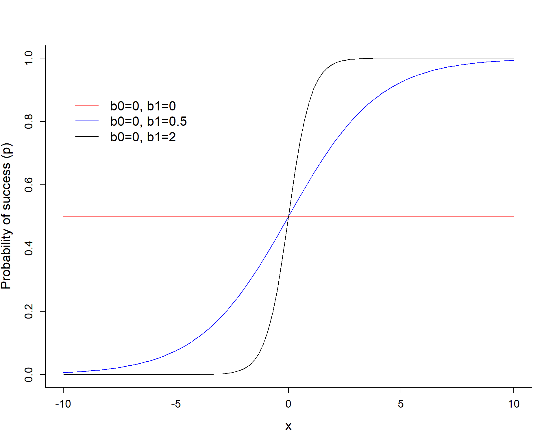
The slope coefficient \(\beta_1\) controls how quickly we transition from 0 to 1.
\[logit(p_i) = log(\frac{p_i}{1-p_i}) = \beta_0 + \beta_1x_i\]
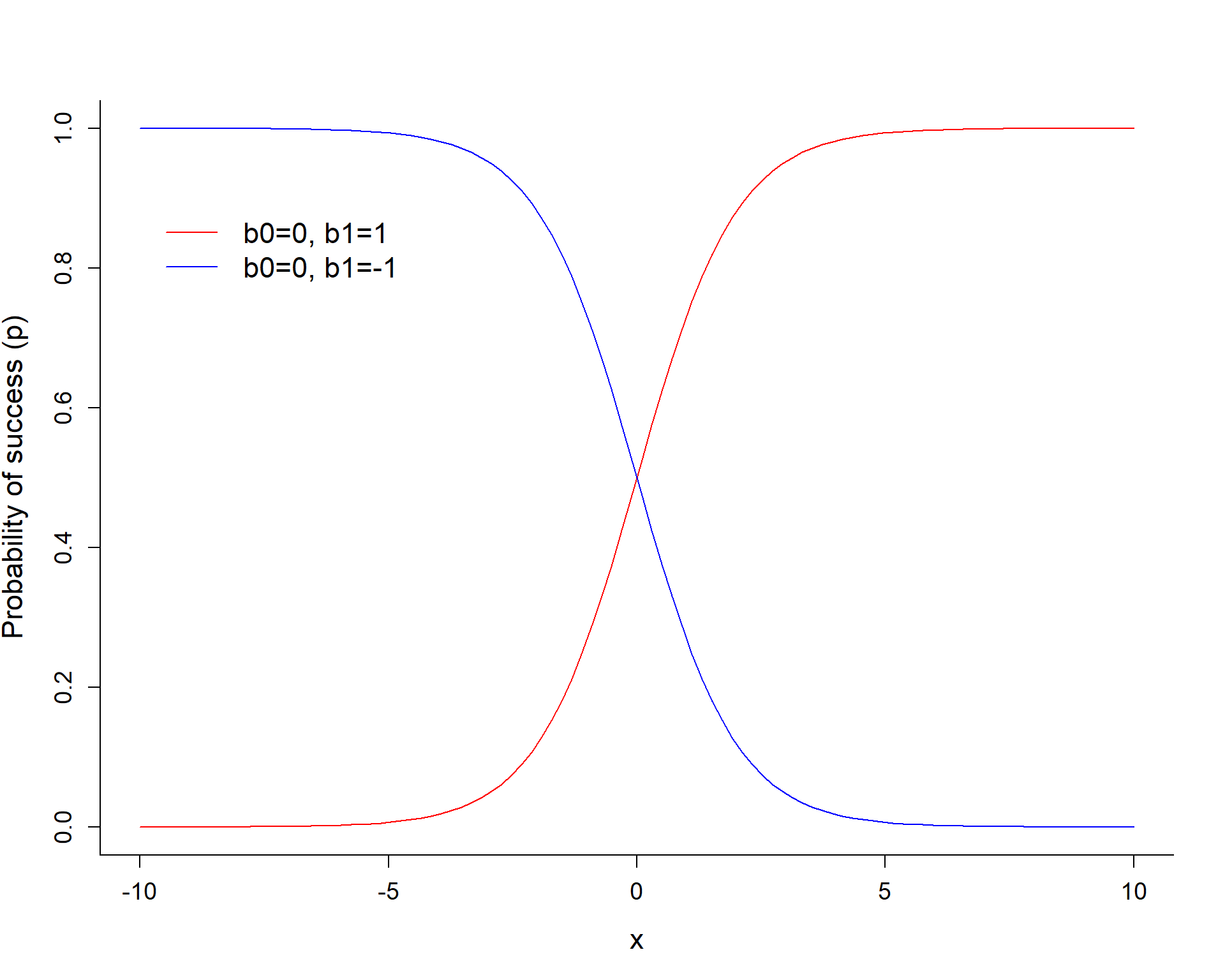
The sign of \(\beta_1\) determines if \(p\) increases or decreases as we increase \(X\) .
\[logit(p_i) = log(\frac{p_i}{1-p_i}) = \beta_0 + \beta_1X_i\]
\(\beta_0\) controls the height of the curve when \(X=0\) .
Gives the log odds of detection when all predictor variables = 0
\(E[Y_i|X_i =0] = \frac{exp(\beta_0)}{1+exp(\beta_0)}\) (equals 1/2 if \(\beta_0 = 0)\) .
Sightability Surveys: Minnesota Moose
124 trials, 2005-2007
\(n_0\) = 65 missed groups\(n_1\) = 59 observed groups
Binary observations, \(Y_i = 0 \mbox{ (missed) or } 1 \mbox{ (seen)}\) .
Covariates thought to influence detection.
\[Y_i | X_i \sim Bernoulli(p_i)\]
\[logit(p_i) = \log\left(\frac{p_i}{1-p_i}\right) = \beta_0 + \beta_1 voc_i\]
Assumptions:
observations are independent
log odds is a linear function of \(voc\)
mean and variance depend on \(voc\)
\(E[Y_i|X_i] = p_i; Var[Y_i|X_i] = p_i(1-p_i)\) with:
\(p_i = \frac{\exp(\beta_0 + \beta_1 voc_i)}{1+\exp(\beta_0 + \beta_1 voc_i)}\)
<- glm (observed~ voc, data= exp.m, family= binomial ())summary (mod1)
Call:
glm(formula = observed ~ voc, family = binomial(), data = exp.m)

Coefficients:
             Estimate Std. Error z value Pr(>|z|)
(Intercept)  1.759933   0.460137   3.825 0.000131 ***
voc         -0.034792   0.007753  -4.487 7.21e-06 ***
---
Signif. codes:  0 '***' 0.001 '**' 0.01 '*' 0.05 '.' 0.1 ' ' 1

(Dispersion parameter for binomial family taken to be 1)

    Null deviance: 171.61  on 123  degrees of freedom
Residual deviance: 147.38  on 122  degrees of freedom
AIC: 151.38

Number of Fisher Scoring iterations: 4
(Intercept)         voc
 1.75993309 -0.03479153
Regression coefficient for voc (visual obstruction) = -0.039.
The log odds of being detected decreases by 0.039 per unit increase in visual obstruction
The odds of being detected decreases by a factor of exp(0.039) = 0.96 per unit increase in visual obstruction
Intercept = 2.12 = log(odds) of detection when VOC = 0.
# p(Y=1|voc=0) = exp(coef(mod1)[1])/(1+exp(coef(mod1)[1])) plogis (coef (mod1)[1 ])
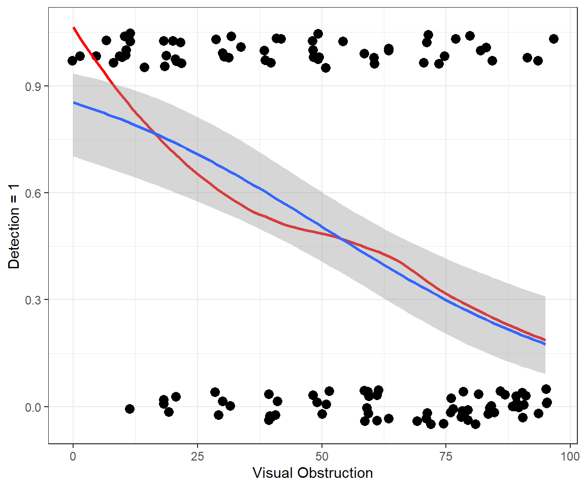
We see roughly 85% of moose if there is no visual obstruction.
ggplot (exp.m, aes (voc,observed))+ theme_bw () + geom_point (position = position_jitter (w = 2 , h = 0.05 ), size= 3 ) + xlab ("Visual Obstruction" ) + geom_smooth (se= F, colour= "red" ) + stat_smooth (method= "glm" , method.args = list (family = "binomial" ))+ ylab ("Detection = 1" )
$ year<- as.factor (exp.m$ year)<- glm (observed~ voc+ year, data= exp.m, family= binomial ())summary (mod2)
Call:
glm(formula = observed ~ voc + year, family = binomial(), data = exp.m)

Coefficients:
             Estimate Std. Error z value Pr(>|z|)
(Intercept)  2.453203   0.622248   3.942 8.06e-05 ***
voc         -0.037391   0.008199  -4.560 5.11e-06 ***
year2006    -0.453862   0.516567  -0.879   0.3796
year2007    -1.111884   0.508269  -2.188   0.0287 *
---
Signif. codes:  0 '***' 0.001 '**' 0.01 '*' 0.05 '.' 0.1 ' ' 1

(Dispersion parameter for binomial family taken to be 1)

    Null deviance: 171.61  on 123  degrees of freedom
Residual deviance: 142.23  on 120  degrees of freedom
AIC: 150.23

Number of Fisher Scoring iterations: 4
(Intercept)         voc    year2006    year2007
 2.45320264 -0.03739118 -0.45386154 -1.11188432
Year 2005: \(log(p_i/(1-p_i)) = 2.45 -0.037VOC\)
Year 2006: \(log(p_i/(1-p_i)) = 2.45 -0.037VOC -0.45\)
So,-0.45 gives the difference in log odds between years 2005 and 2004 (if we hold VOC constant).
exp(-0.45) = 0.63 = odds ratio (year 2006 to year 2005)
odds ratio = \(\frac{p_{2006}/(1-p_{2006})}{p_{2005}/(1-p_{2005})} = 0.63\)
Supporting Theory
The estimates of \(\beta\) are maximum likelihood estimates, found by maximizing:
\[L(\beta; y, x) = \prod_{i=1}^{n}p_i^{y_i}(1-p_i)^{1-y_i}, \text{ with}\]
\[p_i = \frac{e^{\beta_0 + \beta_1x_1 + \ldots \beta_kx_k}}{1+e^{\beta_0 + \beta_1x_1 + \ldots \beta_kx_k}}\]
Remember, for large samples, \(\hat{\beta} \sim N(\beta, \Sigma)\) .
We can use this theory to conduct tests (z-statistics and p-values in output by the summary function) and to get confidence intervals.
logit\((p) = \beta_0 + \beta_1x_1 + \ldots \beta_kx_k\) is more “Normal” than \(p\)
Confidence intervals
Generate confidence intervals for logit(\(p\) ), then back-transform to get confidence intervals for \(p\)
Ensures the confidence intervals will live on the (0,1) scale
Intervals will not be symmetric
If confidence limits for \(\beta\) include 0 or confidence limits for \(exp(\beta)\) include 1, then we do not have enough evidence to say that years differ in their detection probabilities.
(Intercept)         voc    year2006    year2007
 2.45320264 -0.03739118 -0.45386154 -1.11188432
(Intercept)         voc    year2006    year2007
0.622247867 0.008199483 0.516567443 0.508269279
exp (rep (0.006879 , 2 )+ c (- 1.96 , 1.96 )* 0.53664 ) # exp(beta +/-1.96SE)
95% Confidence interval for odds ratio = (0.35, 2.88) includes 1 (not statistically significant)
Confint
                  2.5 %     97.5 %
(Intercept)  1.30341777  3.7586692
voc         -0.05448153 -0.0221268
year2006    -1.48479529  0.5516852
year2007    -2.14380706 -0.1382692
These are profile-likelihood based confidence intervals based on “inverting” the likelihood ratio test (see Maximum Likelihood notes).
    2.5 %    97.5 %
0.2265487 1.7361764
Profile-likelihood based intervals should have better statistical properties with small data sets (better coverage rates).
Hosmer-Lemeshow test
Group Observations by deciles of their predicted values to form groups, then calculate the expected and observed number of successes and failures for each group.
\[\chi^2 = \sum_{i=1}^{n_g}\frac{(O_i-E_i)^2}{E_i} \sim \chi^2_{g-2}\]
where \(g\) = number of groups.
library (ResourceSelection)hoslem.test (exp.m$ observed, fitted (mod1), g= 8 )
    Hosmer and Lemeshow goodness of fit (GOF) test

data:  exp.m$observed, fitted(mod1)
X-squared = 3.2505, df = 6, p-value = 0.7768
Goodness-of-fit
Can adapt our general approach for testing goodness-of-fit using Pearson residuals (\(r_i\) )
\[r_i = \frac{Y_i-E[Y_i|X_i]}{\sqrt{Var[Y_i|X_i]}}\]
\(E[Y_i|X_i] = p_i\) = \(\frac{exp(\beta_0 + \beta_1x_1+\ldots \beta_kx_k)}{1+exp(\beta_0 + \beta_1x_1+\ldots \beta_kx_k)}\) \(Var[Y_i|X_i] =\) \(p_i(1-p_i)\)
See textbook for an implementation of this test…
Residual plots
    Test stat Pr(>|Test stat|)
voc   -35.056                1
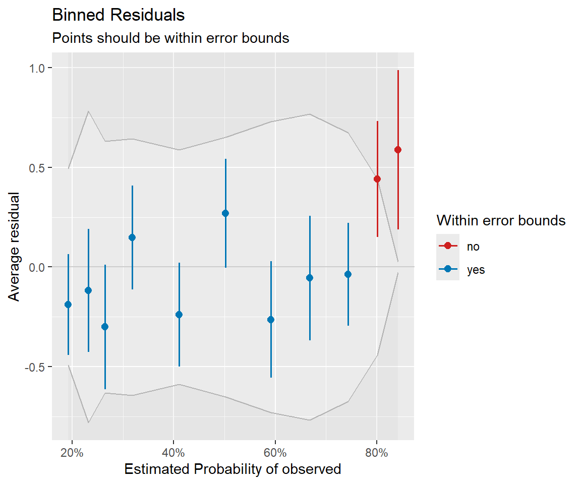
Binned residual plot
<- performance:: binned_residuals (mod1)plot (binplot)
Likelihood ratio tests
We can again use difference in deviences (equivalent to likelihood ratio tests) to compare full and reduced models.
drop1 (mod2, test= "Chisq" )
Single term deletions

Model:
observed ~ voc + year
       Df Deviance    AIC     LRT  Pr(>Chi)
<none>      142.23 150.23
voc     1   168.20 174.20 25.9720 3.464e-07 ***
year    2   147.38 151.38  5.1558   0.07593 .
---
Signif. codes:  0 '***' 0.001 '**' 0.01 '*' 0.05 '.' 0.1 ' ' 1
voc is an important predictor, the importance of year is less clear.
ANOVA function (car package)
Or use Anova in car package
Analysis of Deviance Table (Type II tests)

Response: observed
     LR Chisq Df Pr(>Chisq)
voc   25.9720  1  3.464e-07 ***
year   5.1558  2    0.07593 .
---
Signif. codes:  0 '***' 0.001 '**' 0.01 '*' 0.05 '.' 0.1 ' ' 1
AIC
We can compare nested or non-nested models using the AIC function
     df      AIC
mod1  2 151.3824
mod2  4 150.2266
Probability Scale
We can also summarize models by getting predicted values: \(P(\mbox{detect animal} | \mbox{voc})\) :
\(logit(p_i) = \beta_0 + \beta_1x_1 + \ldots \beta_kx_k\)
\(P(Y_i = 1 | X= x) = p_i = \frac{e^{\beta_0 + \beta_1x_1 + \ldots \beta_kx_k}}{1+e^{\beta_0 + \beta_1x_1 + \ldots \beta_kx_k}}\) (inverse logit)
We can use predict(model, newdata=, type="link", se=TRUE) to get predictions on logit scale.
Then use plogis(p.hat$fit +/- 1.95*p.hat$se.fit) to transform the limits back to the probability scale.
A note on model visualization
Model 2: observed \(\sim\) voc + year is additive on the logit scale
Differences in logit(\(p\) ) among years will not depend on voc
Differences in \(p\) , will however, depend on voc!
See: Section 16.6.3 in the book
Can always create your own “effect” plots by calculating predicted values for different combinations of your predicted values
Can use the effects package or ggeffects to do something similar
Effect plots on probability scale
Using effects or ggeffects package:
Fixes all continuous covariates (other than the one of interest) at their mean values
Categorical predictors: averages predictions on link scale, weighted by proportion of data in each category, then back transforms to probability scale
These are refereed to as marginal predictions by ggeffects
Effect plots
library (ggeffects); library (patchwork)<- plot (ggeffect (mod2, "year" ))<- plot (ggeffect (mod2, "voc" ))+ p2
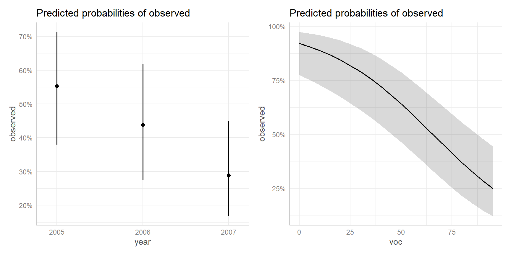
Adjusted plots
Instead of averaging predictions across years, we could set year to a specific value. This leads to adjusted plots .
library (ggeffects); library (patchwork)<- plot (ggpredict (mod2, "year" ))<- plot (ggpredict (mod2, "voc" ))+ p2
JAGS
Will use a similar structure as we used for count models:
A linear predictor, \(\eta = \beta_0 + \beta_1x_1\) (\(x_1\) = voc)
\(p_i = g^{-1}(\eta) = \frac{e^{\eta_i}}{1+e^{\eta_i}}\)
\(Y[i] \sim\) dbin(p[i],1)
Gelman’s recommendations (see arxiv.org/pdf/0901.4011.pdf):
scale continuous predictors so they have mean 0 and sd = 0.5
using a non-informative Cauchy prior dt(0, pow(2.5,-2), 1)
In class exercise: adapt the JAGS code for fitting mod1 (voc only) to allow fitting of mod2 (voc + year).