Models for Data with Zero Inflation
Learning Objectives
- Be able to fit models to response data with lots of zeros (hurdle and zero-inflated models)
- Be able to describe these models and their assumptions using equations and text and match parameters in these equations to estimates in computer output.
Zero-Inflation
Zero-inflation deals with response data, \(Y_i\), not predictors, \(X_i\).
Zero inflation has received the most attention for count data.
Also relevant to:
- Binary data (occupancy models, Kery Ch 20)
- Continuous data (e.g., Friederichs et al. 2011. Oikos 120:756-765)
Abundance Data and Zero Inflation

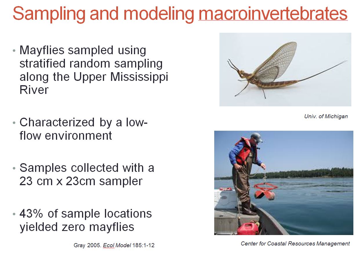
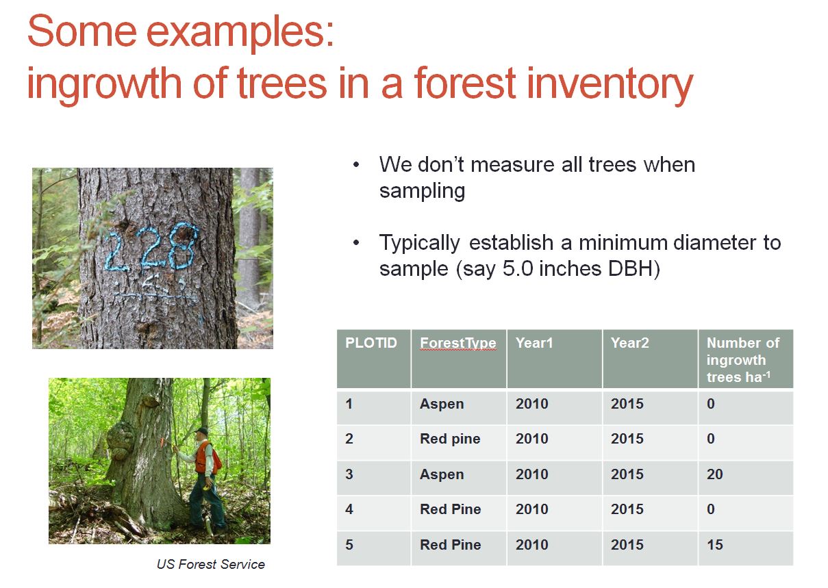
Top 4 reasons why you might get a 0 when counting critters?
- Sites are not suitable for the species
- Density effects: a site is suitable, but unoccupied
- Design errors: sampling for too short of a time period, or during the wrong times
- Observer error: some species are difficult to identify/detect
Picture (and next two slides) provided by Matt Russell (formally in FR)
Zeros and common statistical distributions
Count data:
- Poisson and Negative Binomial distributions allow for zeros, i.e., \(P(Y=0) \ne 0\).
- Need to ask, are there more zeros than expected if the data followed Poisson(\(\lambda_i\)) or NegBin(\(\mu_i, \theta\)) distributions?
For continuous data:
- We do not expect a “piling” up of zeros
How can we determine if we have excess zeros?
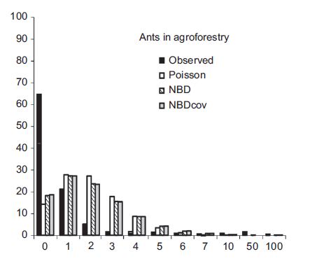
- Compare predicted and observed number of 0’s (could use for a Goodness-of-fit test)
See textbook (and R code for an example)!
Modeling Zero-Inflated Data
What do we do if we have zero-inflation?
- Hurdle models: model presence-absence (0 non-zero) and counts given presence
- Mixture models: allow for multiple ways to get a 0
For the in-class exercise, we will focus on the latter approach.
- Review interpretation of parameters in logistic and count-based regression models
- Showcase features of Bayesian implementations (using MCMC to average over / integrate out unknowns)
Hurdle Models
Group all 0’s into a single category:
Hurdle: positive counts arise if you exceed some threshold (with probability \(\pi\))
Hurdle Models
- Presence-absence subcomponent:
\(Z_i =\left\{\begin{array}{ll} \mbox{0 when } y=0 & \mbox{occurs with probability } (1-\pi) \\ \mbox{1 when } y>0 & \mbox{occurs with probability } \pi \end{array}\right\}\)
Can model \(Z_i\) using using logistic regression to allow presence-absence to depend on covariates
- Count model subcomponent:
Model the non-zero data (using truncated distribution models)
- Poisson or negative binomial, modified to exclude the possibility of a 0
Can do this in two steps or use a single modeling framework (see Hurdle models Ch 11.5 in Zuur et al).
Truncated Distributions
\(P(Y = y | Y > 0) = \frac{P(Y=y)}{P(Y>0)}= \frac{f(y)}{(1-f(0))}\)
Remember, P(A|B) = P(A and B)/P(B)
A truncated Poisson would look like…
\[P(Y=y | y > 0) = \frac{\frac{e^{-\lambda}\lambda^y}{y!}}{1-e^{-\lambda}}\]
We can incorporate covariates, using: log(\(\lambda) = \beta_0 + \beta_1x +\ldots\)
However, note:
- \(E[Y|X] \ne \lambda_i\) (due to truncation of the Poisson and zero-inflation)
- See Zuur et al. p. 288 for expressions for \(E[Y|X]\) and \(Var[Y|X]\)
Truncated Distributions for Continuous Data
- Log-normal, gamma distributions live on (0, \(\infty\)) (so no need to truncate these)
- Or, can use truncated distributions (e.g., Normal) \(= \frac{f(y)}{1-F(0)}\) where \(F(y) = P(Y \le y)\)
Which function in R is used to determine \(f(Y)\)? dnorm!
Which function in R is used to determine \(F(Y)\)? pnorm!
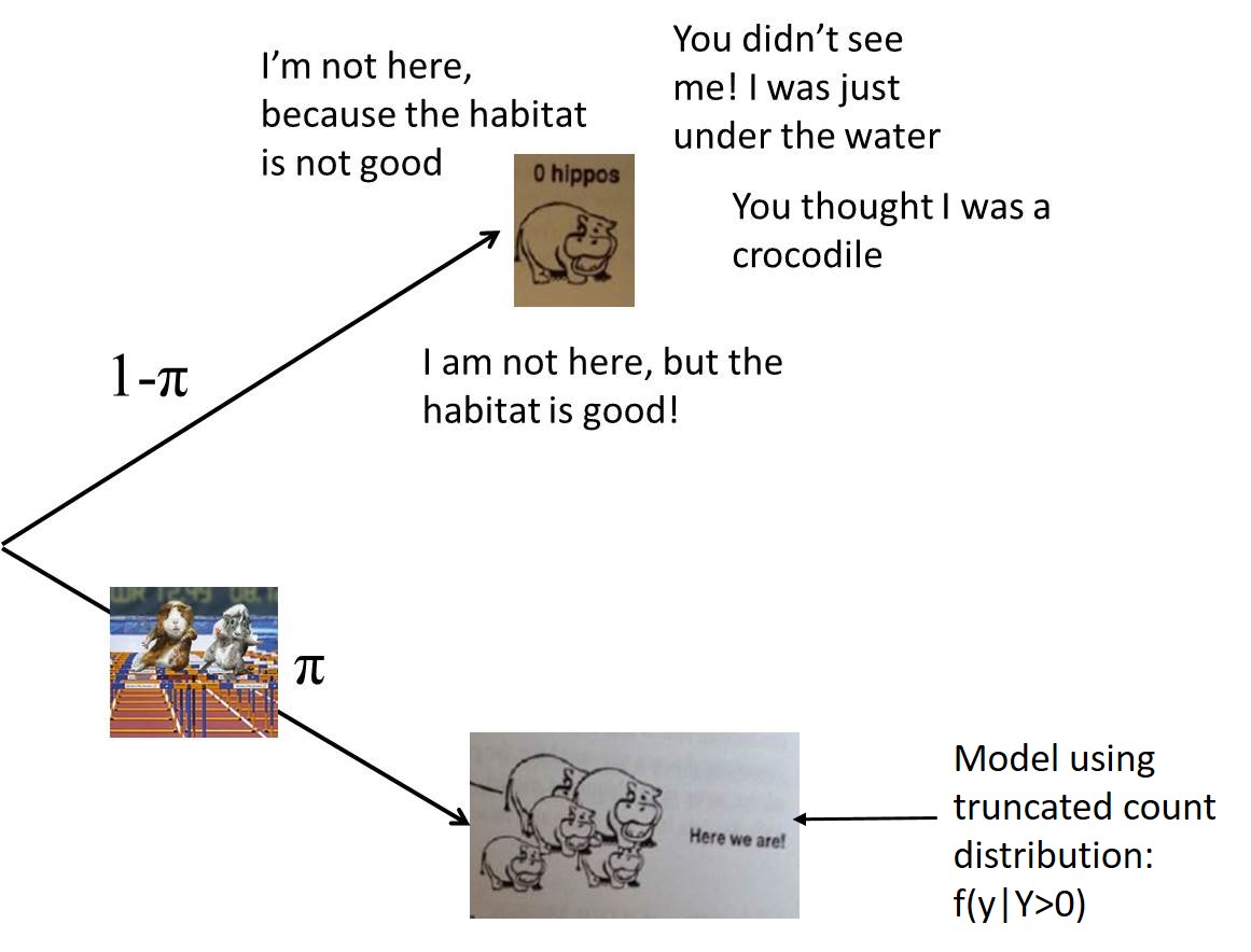
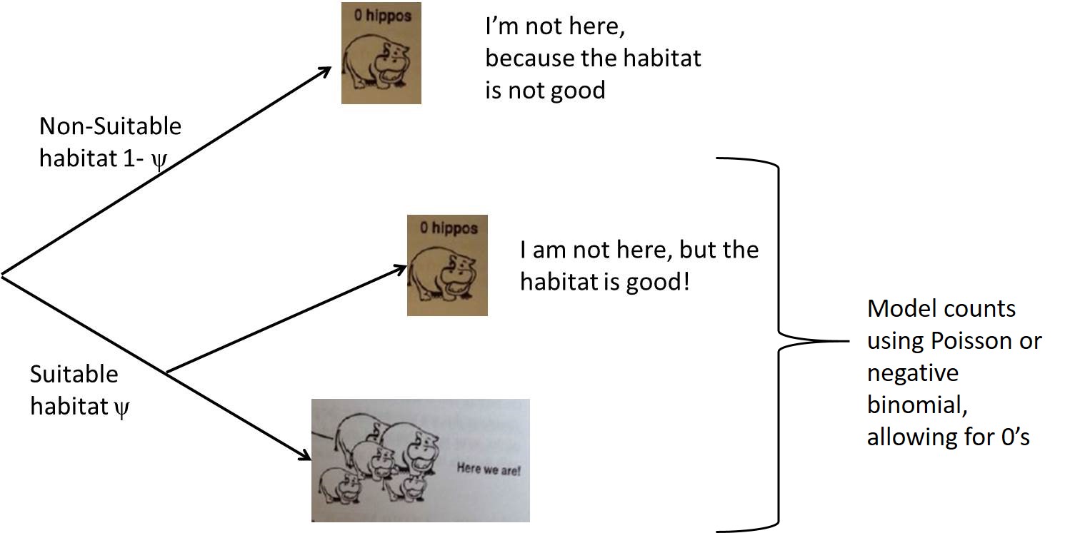
Mixture Model (Kery)
Two ways to get a 0:
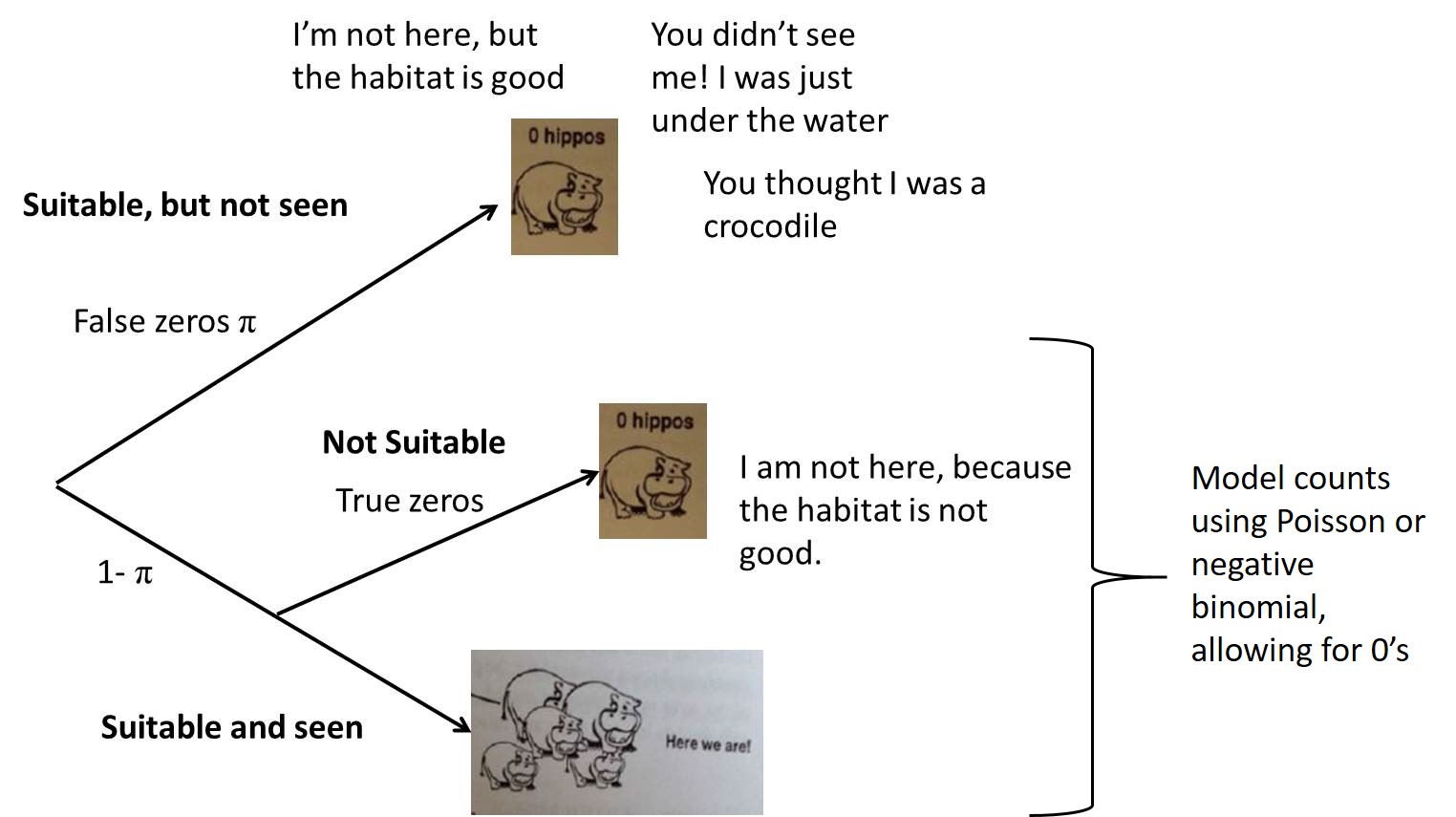
Mixture Models (Zuur et al)
Reality
Zero-inflation:
- Kery suggests we think of the extra zeros as arising from non-suitable habitat
- Zuur et al. suggests we view the extra zeros as suitable habitat where species are not detected
Our assumptions can influence our choice of covariates for the zero-inflation process!
Assigning meaning to the zero-inflation process can in some cases be useful, but it also requires a leap of faith!
Equations
Let:
- \(Z_i\) = 1 if the \(i^{th}\) observation is an inflated 0 (and 0 otherwise).
- \(Y_i\) = the count (response) variable for the \(i^{th}\) observation.
\[\begin{gather} Z_i \sim Bernoulli(p_i) \\ logit(p_i) = \gamma_0 + \gamma_1\tilde{X}_i \end{gather}\]
If \(Z_i = 1\), then \(Y_i = 0\)! If \(Z_i = 0\), then \(Y_i\) has a Poisson distribution!
\[\begin{gather} Y_i| Z_i \sim Poisson((1-Z_i)\lambda_i) \\ \log(\lambda_i) = \beta_0 + \beta_1 X_i \end{gather}\]
We observe \(Y_i\) but we only “partially observe” \(Z_i\) (we don’t know its value when \(Y_i = 0\))
Parameter estimation
Frequentist approaches require that we average over or integrate out any unobserved quantities (whether the observation is an inflated zero or not) to calculate the marginal likelhood of the data.
To calculate the likelihood of the data, we need to determine the probability of getting a count of 0, 1, 2, etc:
\[P(Y_i = y) = \sum_z P(Y_i = y \mid Z_i = z)P(Z_i = z)\] where \(Z_i = 1\) if the \(i^{th}\) observation is an inflated 0 and 0 otherwise.
Bayesian approaches can use MCMC to do this averaging/integration over the unobserved \(Z_i\).
Marginal Likelihood
We can get a 0 in two ways:
- We have an inflated zero with probability \(\pi\)
- We have a non-inflated zero with probability \((1-\pi)f(0)\)
\(P(Y = 0) = \pi + (1-\pi)f(0)\) (i.e., the sum of these two probabilities).
Non-zero responses occur with probability: \((1-\pi)f(y)\)
Marginal Likelihood: Zero-inflated Poisson (ZIP)
Probability Mass Function: \(f(y) = \frac{e^{-\lambda}\lambda^y}{y!}\)
ZIP model (Zuur):
\(P(Y=y) = f(y) =\left\{\begin{array}{ll} \pi + (1-\pi)e^{-\lambda} & \mbox{if } y = 0\\ (1-\pi)\frac{e^{-\lambda}\lambda^y}{y!} & \mbox{if } y = 1, 2, 3, \ldots \end{array} \right.\)
ZINB model: Zero-inflated Negative Binomial
Probability Mass Function: \(f(y) = {y+\theta-1 \choose y}\left(\frac{\theta}{\mu+\theta}\right)^{\theta}\left(\frac{\mu}{\mu+\theta}\right)^y\)
ZINB model (Zuur et al):
\(f(y) =\left\{ \begin{array}{ll} \pi + (1-\pi)\left(\frac{\theta}{\mu+\theta}\right)^\theta & \mbox{if } y = 0\\ (1-\pi){y+\theta-1 \choose y}\left(\frac{\theta}{\mu+\theta}\right)^{\theta}\left(\frac{\mu}{\mu+\theta}\right)^y & \mbox{if } y = 1, 2, 3, \ldots \end{array} \right.\)
We can fit models using the zeroinfl function in the pscl package in R:
- Hurdle model and mixture models with both the Poisson and Negative Binomial distributions (see in class exercise)
Can also code models in JAGS or fit using the glmmTMB package (which allows one to include random effects).
ZIP model: Zero-inflated Poisson
Zuur and zeroinfl function in pscl R package:
- Parameterizes in terms of \(\pi\) = the probability of a zero-inflated response
Kery (and my JAGS implementation):
- Parameterizes in terms of \(\psi = 1- \pi\) = the probability of a NON zero-inflated response
ZIP model (Zuur and zeroinfl):
\(P(Y=y) = f(y) =\left\{\begin{array}{ll} \pi + (1-\pi)e^{-\lambda} & \mbox{if } y = 0\\ (1-\pi)\frac{e^{-\lambda}\lambda^y}{y!} & \mbox{if } y = 1, 2, 3, \ldots \end{array} \right.\)
ZIP model (Kery):
\(P(Y=y) = f(y) =\left\{\begin{array}{ll} 1-\psi + \psi e^{-\lambda} & \mbox{if } y = 0\\ \psi\frac{e^{-\lambda}\lambda^y}{y!} & \mbox{if } y = 1, 2, 3, \ldots \end{array} \right.\)
zeroinfl versus Kery / JAGS
Remember:
zeroinf: models probability of a zero-inflated response (i.e., “false” zero) = \(\pi_i\)- Kery: models the probability of a NON zero-inflated response (i.e., probability of a “true” zero or a count > 0) = \(\psi_i\)
As a result, the sign of the coefficients will differ between the two approaches.
Model Comparisons
Can compare Poisson, Negative Binomial, Zero-inflation models
- Using AIC
- Graphs of observed vs expected proportion of zeros in a dataset
- Graphs of the sample mean–variance relationship.
My experience, and that of others, is that a Negative Binomial model (without zero-inflation) often “wins” (but not always)
- See Warton (2005) on Canvas, as well as Gray (2005), Sileshi (2008)
Also, zero-inflated negative binomial models can sometimes be difficult to fit (past homework problem)
See comments on this blog