Linear Mixed Effects Models

FW8051 Statistics for Ecologists

Learning objectives

• Be able to identify when to use a mixed model

• Learn how to implement mixed models in R/JAGs when the response is Normally distributed (linear mixed effect models, lme)

• Be able to describe models and their assumptions using equations and text and match parameters in these equations to estimates in computer output.

Next chapter:

• Learn how to implement mixed models in R/JAGs for count, presence absence data (generalized linear mixed effect models, glmms)
• Generalized Estimating Equations for count and presence-absence data

Selenium and Fish

library(Data4Ecologists) # for data
data(Selake)

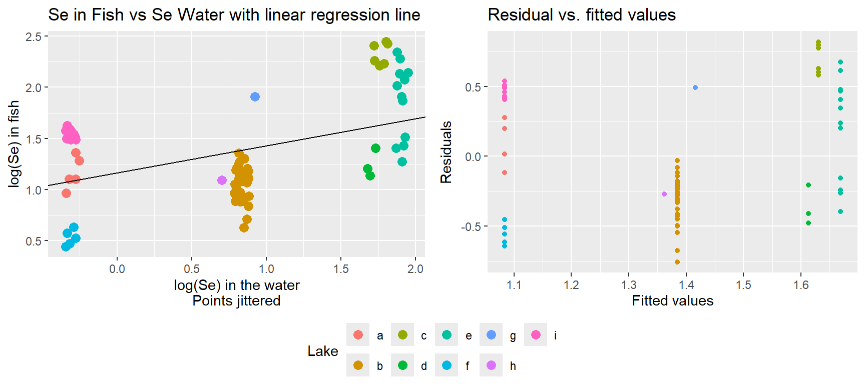
Selenium, Se, a bi-product of burning coal is measured in…

• A set of 9 lakes
• 1 to 34 fish in each lake (total of 83 observations)

Goal: determine the relationship between mean (log) Se in lake and mean (log) Se in fish.

Selenium Example

What are the consequences of ignoring the fact that we have multiple observations from each lake?

• If we use linear regression (assuming independence), our SE’s will be too small (observations from the same lake are not independent)

What strategies might we use to analyze these data?

Note: our main question involves a predictor-response relationship in which the predictor is constant within each cluster or sample unit

Selenium Example

Strategies:

• Fit a linear regression model, but use a cluster-level bootstrap for inference

• Calculate averages of \(Y\) for each cluster, then fit linear regression models to these averages (will have 1 observation per cluster)

• Use a mixed model with a random intercept for each cluster (i.e., lake)

Lets do this!

Mixed models

When to use a mixed model

When you have more than one measurement on the same observational unit

• Multiple observations per lake, animal, study site, etc.

Experiments or surveys with multiple sizes of sample units

• Split-plot designs (treatments applied to whole plots and subplots)
• Cluster samples (samples of households, individuals within households)

When you want to generalize to a larger population of sample units

• Fixed effects: allow inference to only the sample units in the data set
• Random effects: allow us to generalize to a population of sample units by assuming cluster-specific regression parameters come from a common distribution

Multi-level, Mixed Effects, or Hierarchical models

Key features:

• Regression parameters vary by cluster (e.g., population, individual animal, etc.)

• Regression parameters are assumed to come from a common probability distribution (usually Normal)

Why are they so popular:

• Many ecological data sets are hierarchically structured data (e.g., wolves in packs, populations)

• Allows partitioning variance into different components (e.g., variance among individuals, within-individuals)

• Provides a framework for modeling data where the independence assumption is violated

Pines data (book example)

Study objective: investigate tradeoffs between growth rate, size, and lifespan of Mountain pines (Pinus montana) in Switzerland (Bigler, 2016).

Is it better to grow quick but die young? Grow more slowly and live longer?

Sample units:

• 160 dead standing trees sampled at 20 sites

Variables:

• dbh = diameter at breast height (size of tree)
• maximum age (i.e., lifespan)
• Aspect of study site

RIKZdat

Sampling Effort:

• 9 beaches (high, medium, low exposure)
• 5 stations at each beach.

Interest lies in modeling:

• Richness = species richness (number of species counted).

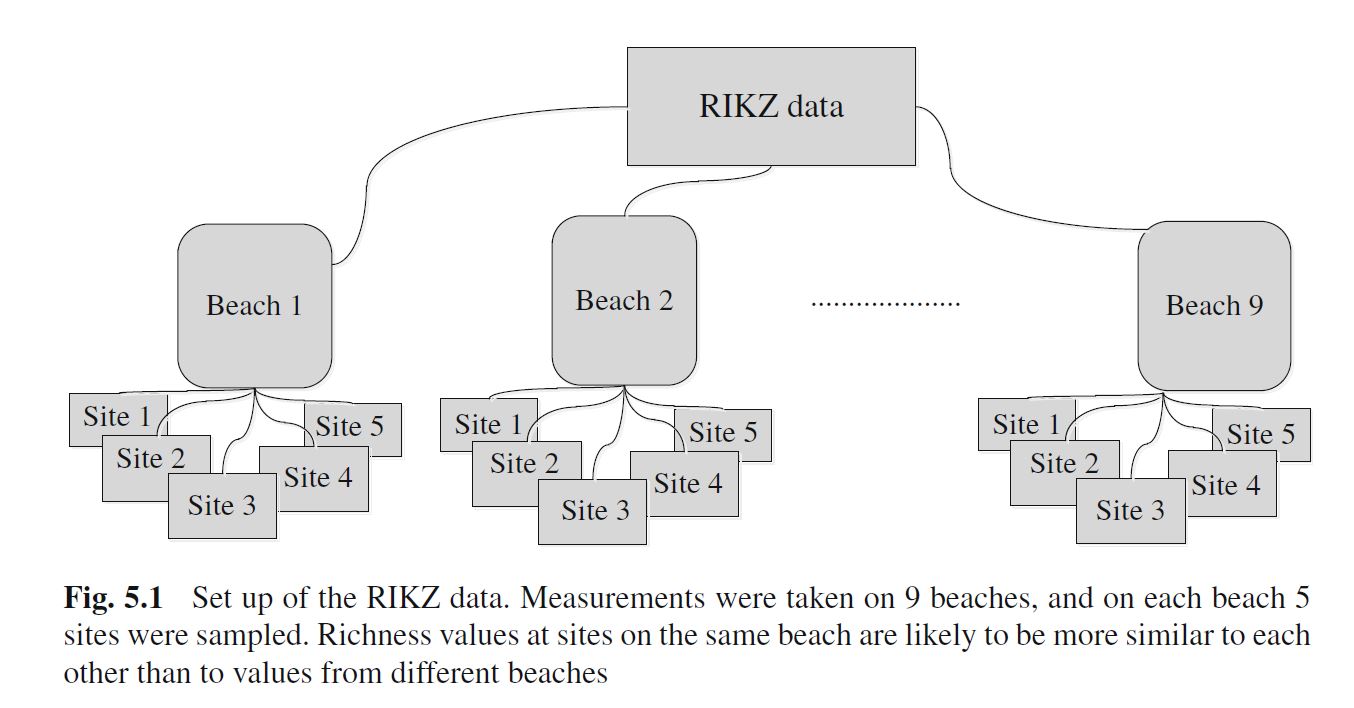
Using macro-fauna and abiotic variables:

• Exposure = low or high exposure to waves, length of surf zone, slope, grain size, and depth of the anaerobic layer
• NAP = height of the sampling station compared to mean tidal level

Linear regression assumes that observations are independent. Is that reasonable in this case?

• 2 observations from the same beach may be more alike than 2 observations taken from 2 different beaches.

• \(\Rightarrow\) observations from the same beach are likely correlated

Multi-level model

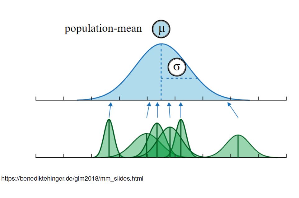
Think of models at 2 levels:

• Level 1: model the how individual observations vary within a cluster

• Level 2: model how (cluster-specific) parameters, in the level-1 model, vary (across clusters)

2-stage multi-level modeling approach

Stage 1 (level 1 model):

• Build a separate model for each cluster (beach)
• Only consider variables that are NOT constant within a cluster

Stage 2 (level 2 model):

• Treat the coefficients from stage 1 as `data’
• Model the coefficients as a function of variables that are constant within a cluster

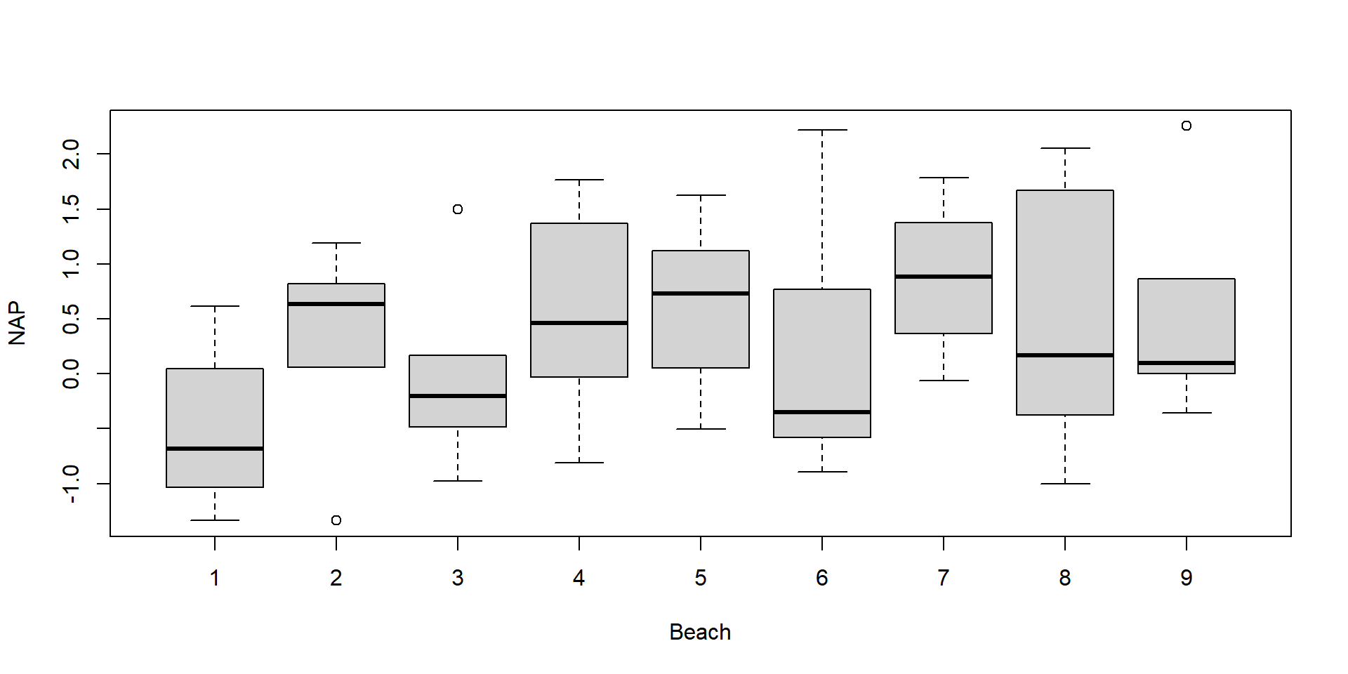
Can be useful exploratory approach when you have lots of data for each cluster, but few clusters

RIKZdat

NAP is a “level-1” covariate (it varies within each cluster)

RIKZdat

exposure is a “level-2” covariate (it is constant within a cluster)

xtabs(~ exposure + Beach, data=RIKZdat)

        Beach
exposure 1 2 3 4 5 6 7 8 9
      8  0 5 0 0 0 0 0 0 0
      10 5 0 0 0 5 0 0 5 5
      11 0 0 5 5 0 5 5 0 0

# Only 1 beach with lowest exposure level: modify to have 2 categories
RIKZdat$exposure.c<-"High"
RIKZdat$exposure.c[RIKZdat$exposure%in%c(8,10)]<-"Low"

2-Stage approach

Let \(R_{ij}\) = the species richness for the \(j^{th}\) sample on the \(i^{th}\) beach (note: we now need two subscripts!)

Level 1 model: model for observations within each cluster (i.e., for each beach)

\(R_{ij} = \beta_{0i} + \beta_{1i}NAP_{ij} + \epsilon_{ij}\); (\(j = 1, 2, \ldots, 5\) observations for each Beach)

Each beach has its own intercept \(\beta_{0i}\) and slope \(\beta_{1i}\)

Modified R code

RIKZdat$NAPc = RIKZdat$NAP-mean(RIKZdat$NAP) #center NAP variable   
Beta<-matrix(NA, 9,2) # to hold slope and intercepts    
Exposure<-matrix(NA,9,1) # to hold exposure level for each beach    
for(i in 1:9){  
  Mi<-lm(Richness~NAPc, data=subset(RIKZdat, Beach==i)) 
  Beta[i,]<-coef(Mi)    
  Exposure[i]<-subset(RIKZdat, Beach==i)$exposure.c[1]  
}   
betadat <- data.frame(Beach = 1:9, intercept = Beta[,1], 
                      slope = Beta[,2], exposure.c = Exposure)

Note: I have centered the NAP variable

• Makes intercept more meaningful = \(R_{ij}\) at the mean value of NAP
• Helps avoid numerical problems and identifiability problems due to correlation of \(\hat{\beta}_{0i}\) and \(\hat{\beta}_{1i}\)

This gives us a data frame of coefficients and level-2 predictors for a level-2 model:

betadat

  Beach intercept      slope exposure.c
1     1 10.692614 -0.3718279        Low
2     2 11.893999 -4.1752712        Low
3     3  2.790385 -1.7553529       High
4     4  2.653600 -1.2485766       High
5     5  9.688335 -8.9001779        Low
6     6  3.841864 -1.3885120       High
7     7  2.992969 -1.5176126       High
8     8  4.293257 -1.8930665        Low
9     9  5.263276 -2.9675304        Low

For a tidyverse solution - see book/R code.

library(ggplot2); library(patchwork)
g1 <-ggplot(betadat, aes(exposure.c, intercept)) + geom_point() 
g2 <-ggplot(betadat, aes(exposure.c, slope)) + geom_point() 
g1+g2

Level-2 model

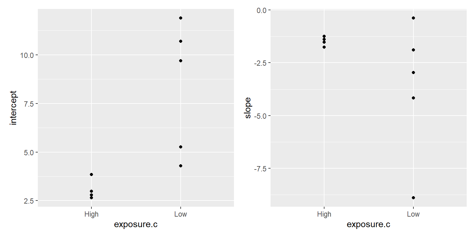
Model for the slope and intercept parameters (analyze the summary statistics, \(\hat{\beta}_{0i}, \hat{\beta}_{1i})\) using level-2 predictors (ones that are constant within a cluster)

• \(\hat{\beta}_{0i} = \beta_0 + \gamma_{0}Exposure_i+b_{0i}\)
• \(\hat{\beta}_{1i} = \beta_1 + \gamma_{1}Exposure_i + b_{1i}\)

For now, ignore the fact that the variability of \(b_{0i}, b_{1i}\) seems to depend on exposure level (“low”, “high”).

Level-2 Model: Intercepts

summary(lm(intercept ~ exposure.c, data = betadat))

Call:
lm(formula = intercept ~ exposure.c, data = betadat)

Residuals:
    Min      1Q  Median      3Q     Max 
-4.0730 -0.4161 -0.0767  1.3220  3.5277 

Coefficients:
              Estimate Std. Error t value Pr(>|t|)  
(Intercept)      3.070      1.291   2.378   0.0491 *
exposure.cLow    5.297      1.732   3.058   0.0184 *
---
Signif. codes:  0 '***' 0.001 '**' 0.01 '*' 0.05 '.' 0.1 ' ' 1

Residual standard error: 2.582 on 7 degrees of freedom
Multiple R-squared:  0.5719,    Adjusted R-squared:  0.5107 
F-statistic: 9.349 on 1 and 7 DF,  p-value: 0.01838

Level-2 Model: Slopes

summary(lm(slope ~ exposure.c, data = betadat))

Call:
lm(formula = slope ~ exposure.c, data = betadat)

Residuals:
    Min      1Q  Median      3Q     Max 
-5.2386 -0.2778  0.0890  0.6940  3.2897 

Coefficients:
              Estimate Std. Error t value Pr(>|t|)
(Intercept)     -1.478      1.229  -1.202    0.268
exposure.cLow   -2.184      1.649  -1.325    0.227

Residual standard error: 2.458 on 7 degrees of freedom
Multiple R-squared:  0.2005,    Adjusted R-squared:  0.08625 
F-statistic: 1.755 on 1 and 7 DF,  p-value: 0.2268

Putting things together: Composite Equation

Level-1 Model:

• \(R_{ij} = \beta_{0i} + \beta_{1i}NAP_{ij} + \epsilon_{ij}\)

Level-2 Model:

• \(\beta_{0i} = \beta_0 + \gamma_{0}Exposure_i+b_{0i}\)
• \(\beta_{1i} = \beta_1 + b_{1i}\)

Substitute into level-1 equation to get the composite equation

\[R_{ij} = (\beta_0 + \gamma_{0}Exposure_i+b_{0i}) + (\beta_1+b_{1i})NAP_{ij} + \epsilon_{ij}\]

\[R_{ij} = (\beta_0 + b_{0i}) + (\beta_1+b_{1i})NAP_{ij} + \gamma_0Exposure_{i} + \epsilon_{ij}\]

\(\Rightarrow\) random intercepts and slopes model (or random coefficients model)

Mixed Models

Rather than use a 2-stage approach, we could just posit a model for the data using random and fixed effects.

Random Intercepts Model:

\[R_{ij} = \beta_0 + b_{0i}+ \beta_1NAP_{ij} + \beta_2Exposure_i + \epsilon_{ij}\] \[b_{0i} \sim N(0,\sigma^2_{b_{0}})\] \[\epsilon_{ij} \sim N(0, \sigma^2_\epsilon)\]

Random Intercepts and Slopes Model:

\[R_{ij} = (\beta_0 + b_{0i}) + (\beta_1+b_{1i})NAP_{ij} + \beta_2Exposure_{i} + \epsilon_{ij}\] \[(b_{0i}, b_{1i}) \sim N(0,D)\] \[\epsilon_{ij} \sim N(0, \sigma^2_\epsilon)\]

Random Intercepts and Slopes Model:

\[R_{ij} = (\beta_0 + b_{0i}) + (\beta_1+b_{1i})NAP_{ij} + \beta_2Exposure_{i} + \epsilon_{ij}\] \[(b_{0i}, b_{1i}) \sim N(0,D)\] \[\epsilon_{ij} \sim N(0, \sigma^2_\epsilon)\]

We can think of \(b_{0i}\) and \(b_{1i}\) as deviations from the average intercept (\(\beta_0\)) and slope (\(\beta_1\)), respectively.

Or, we can think in terms of beach-level intercepts and slopes:

• \(\beta_{0i}=\beta_0+b_{0i}\)
• \(\beta_{1i}=\beta_1 + b_{1i}\), with

• \((\beta_{0i}, \beta_{1i}) \sim MVN(\beta, D)\), with \(\beta = \begin{bmatrix} \beta_0\\ \beta_1 \end{bmatrix}\)

\[R_{ij} = (\beta_{0i}) + (\beta_{1i})NAP_{ij} + \beta_2Exposure_{i} + \epsilon_{ij}\]

Fitting Mixed Effects Models in R

Two popular packages: nlme and lme4:

nlme (older)

• More flexibility for modeling within-cluster correlation and heterogeneity (e.g., time series data, spatial data), but slowly being replaced by other options (e.g., glmmTMB, INLA);
  
• Responses must be Normally distributed

lme4 (newer)

• Better options for fitting non-normal data: generalized linear mixed effects models [GLMMS] for count or binary data
  
• Easier to fit non-nested or ‘crossed’ random effects (e.g., year and Beach if we had many years of data).
  
• Cannot handle within-cluster correlation or heterogeneity

Other Packages

Many others too…see glmm wikidot

Two others that we will consider:

• glmmTMB
• GLMMadaptive

For now, let’s fit the random intercept and random intercept and slope models using the lmer function in the lme4 package!

Random Intercepts Model:

\[R_{ij} = \beta_0 + b_{0i}+ \beta_1NAP_{ij} + \beta_2Exposure_i + \epsilon_{ij}\] \[b_{0i} \sim N(0, \sigma^2_{b_{0}})\] \[\epsilon_{ij} \sim N(0, \sigma^2_\epsilon)\]

Fit this model in R using lmer and identify \(\hat{\beta}_0\), \(\hat{\beta}_1\), \(\hat{\sigma}^2_\epsilon\), \(\hat{\sigma}^2_{b_{0}}\)!

Random Intercepts and Slopes Model:

\[R_{ij} = (\beta_0 + b_{0i}) + (\beta_1+b_{1i})NAP_{ij} + \beta_2Exposure_{i} + \epsilon_{ij}\] \[(b_{0i}, b_{1i}) \sim N(0,D)\]

\[D = \begin{bmatrix} var(b_{0i}) & cov(b_{0i},b_{1i}) \\ cov(b_{0i},b_{1i}) & var(b_{1,i}) \end{bmatrix}\]

\[\epsilon_{ij} \sim N(0, \sigma^2_\epsilon)\]

Fit this model in R and identify the different parameters:

• \(var(\epsilon_{ij}) = \sigma^2\) = 6.50 (variance within a Beach)
• \(var(b_{0i}) = 4.750\) (variance among beach intercepts)
• \(var(b_{1i}) = 3.567\) (variance among beach slopes)
• Cor\((b_{0i}, b_{1i}) = \frac{Cov(b_{0i}, b_{1i})}{\sqrt{var(b_{0i})var(b_{1i})}} = -0.557\)

Model Equations

We can write our models in two ways…

\[R_{ij} = (\beta_0 + b_{0i}) + \beta_1NAP_{ij} + \beta_2Exposure_{i} + \epsilon_{ij}\] \[b_{0i} \sim N(0,\sigma^2_{b_{0}})\] \[\epsilon_{ij} \sim N(0, \sigma^2_\epsilon)\]

\[R_{ij} | b_{0i} \sim N(\mu_i, \sigma^2_\epsilon)\] \[\mu_i = (\beta_0 + b_{0i}) + \beta_1NAP_{ij} + \beta_2Exposure_{i}\] \[b_{0i} \sim N(0,\sigma^2_{b_{0}})\]

With either approach, we have 2 random processes that are both formulated using a Normal distribution.

The latter will more easily translate to other statistical distributions (generalized linear mixed effects models).

Later, we will see that for this model, we can derive the marginal distribution of \(R_{ij}\) and refer to it rather than \(R_{ij} \mid b_{0i}\)

Cluster-specific parameters

• We estimate \(\sigma^2_{b_{0}}\), not the individual \(b_{0i}\)

• Since the \(b_{0i}\) are assumed to be “random”, we “predict” them (similar to “estimating” errors, \(\epsilon_i\) using residuals)

• BLUPS = best linear unbiased predictions (see Book section 18.8 for details on how they are calculated).

If you are a Bayesian, you can ignore the distinction between “prediction” and “estimation”…ALL parameters are random variables!

Demonstration w/ R code.

Fixed versus Random Comparison

Each beach also has its own intercept. What if we modeled Beach using fixed effects? . . .

lm.fe <- lm(Richness~factor(Beach)-1+NAPc, data=RIKZdat)
summary(lm.fe)

Call:
lm(formula = Richness ~ factor(Beach) - 1 + NAPc, data = RIKZdat)

Residuals:
    Min      1Q  Median      3Q     Max 
-4.8518 -1.5188 -0.1376  0.7905 11.8384 

Coefficients:
               Estimate Std. Error t value Pr(>|t|)    
factor(Beach)1   8.9392     1.4301   6.251 3.61e-07 ***
factor(Beach)2  12.0173     1.3690   8.778 2.29e-10 ***
factor(Beach)3   2.5343     1.3796   1.837 0.074716 .  
factor(Beach)4   2.9063     1.3723   2.118 0.041364 *  
factor(Beach)5   8.0409     1.3746   5.850 1.22e-06 ***
factor(Beach)6   3.7161     1.3697   2.713 0.010271 *  
factor(Beach)7   3.5025     1.3934   2.514 0.016705 *  
factor(Beach)8   4.3862     1.3707   3.200 0.002920 ** 
factor(Beach)9   5.1572     1.3731   3.756 0.000629 ***
NAPc            -2.4928     0.5023  -4.963 1.79e-05 ***
---
Signif. codes:  0 '***' 0.001 '**' 0.01 '*' 0.05 '.' 0.1 ' ' 1

Residual standard error: 3.06 on 35 degrees of freedom
Multiple R-squared:  0.8719,    Adjusted R-squared:  0.8353 
F-statistic: 23.82 on 10 and 35 DF,  p-value: 9.56e-13

Fixed versus random

Fixed effects:

• lm.fe <- lm(Richness~factor(Beach)-1+NAPc, data=RIKZdat)
• Each beach has its own intercept which we estimate

Random effects:

• lme.fit<-lme(Richness~NAPc+exposure.c + (1|Beach), data=RIKZdat)
• Each beach has its own intercept
• We further assume \(\beta_{0i} \sim N(\beta_0, \sigma^2_{b_{0}})\) or equivalently \(b_{0i}\sim N(0, \sigma^2_{b_{0}})\)
• We estimate the mean (\(\beta_0\)) and variance (\(\sigma^2_{b_{0}}\)) of the intercepts and “predict” the beach-level intercepts

Downsides to fixed effects model

• Requires estimation of 8 parameters

• Cannot include exposure.c since it is constant for each Beach (and therefore, confounded with the Beach coefficients)

lm.fe2 <- lm(Richness~factor(Beach)-1+NAPc+exposure.c, data=RIKZdat)
coef(lm.fe2)

factor(Beach)1 factor(Beach)2 factor(Beach)3 factor(Beach)4 factor(Beach)5 
      8.939200      12.017303       2.534266       2.906323       8.040936 
factor(Beach)6 factor(Beach)7 factor(Beach)8 factor(Beach)9           NAPc 
      3.716094       3.502535       4.386168       5.157177      -2.492836 
 exposure.cLow 
            NA 

• Random coefficients would require interactions between Beach and NAP (another 8 parameters)

Shrinkage (demonstration in R!)

Shrinkage depends on:

• how variable the coefficients are across clusters
• the degree of uncertainty associated with individual estimates

Predicted values

\[R_{ij}|b_i \sim N(\mu_i, \sigma^2_\epsilon)\] \[\mu_i = (\beta_0 + b_{0i}) + (\beta_1+b_{1i})NAP_{ij} + \beta_2Exposure_{i}\] \[b_i = (b_{0i}, b_{1i}) \sim N(0, D) \text{ with}\] \[D = \begin{bmatrix} var(b_{0i}) & cov(b_{0i},b_{1i}) \\ cov(b_{0i},b_{1i}) & var(b_{1,i}) \end{bmatrix}\]

Subject-Specific (lines for a particular beach):

• \(E[R_{ij} | X_{ij}, b_{i}] = \mu_i = \beta_0 + b_{0i} + (\beta_1 + b_{1i})NAP + \beta_2\)I(exposure=“LOW”)\(_i\)

Subject-Specific (line for a “typical” beach with \(b_{0i} = b_{1i} = 0)\):

• \(E[R_{ij} | X_{ij}, b_{i}] = \beta_0 + \beta_1NAP + \beta_2\)I(exposure=“LOW”)\(_i\)

Population Average (averages over beaches):

• \(E[R_{ij} | X_{ij}] = E(E[R_{ij} | X_{ij}, b_{i}])) = \beta_0 + \beta_1NAP + \beta_2\)I(exposure=“LOW”)\(_i\)

R for a demonstration!

Diagnostics

Random Intercepts and Slopes Model:

\[R_{ij} = (\beta_0 + b_{0i}) + (\beta_1+b_{1i})NAP_{ij} + \beta_2Exposure_{i} + \epsilon_{ij}\] \[(b_{0i}, b_{1i}) \sim N(0,D)\] \[\epsilon_{ij} \sim N(0, \sigma^2_\epsilon)\]

What are our assumptions?

1. Linearity:
   • \(E[Richness|NAP, Exposure]= \beta_0+\beta_1NAP+ \beta_pExposure\)
   • \(E[Richness|NAP, Exposure, b_{0i},b_{1i}]= (\beta_0 + b_{0i}) + (\beta_1+b_{1i})NAP_{ij} + \beta_2Exposure_{i}\)
2. Residuals are Normally distributed with constant variance: \(\epsilon_{ij} \sim N(0, \sigma^2_{\epsilon})\)
3. Beaches are independent
4. \((b_{0i}, b_{1i}) \sim MVN(0, D)\), independent of \(\epsilon_{ij}\)

Diagnostic plots

Plot of within beach residuals, \(\hat{\epsilon_{ij}}\), versus beach-level predictions \({\hat{R}_{ij}} = \hat{\beta}_0 + \hat{b}_{0i} + (\hat{\beta}_1+\hat{b}_{1i})NAP + \hat{\beta}_2(exposure=low)\)

• check_model function offers many more checks

  • QQplots to evaluate Normality of residuals
  • QQplots to evaluate Normality of the random effects
  • Residual versus fitted values and scale-location plot for constant variance
  • Posterior predictive checks
  • Collinearity, influential observations

See R for a demonstration!

Degrees of Freedom (lme)

library(nlme)
lme.fit<-lme(Richness~NAPc+exposure.c, random=~1|Beach, data=RIKZdat)
summary(lme.fit)

Linear mixed-effects model fit by REML
  Data: RIKZdat 
       AIC      BIC    logLik
  240.5538 249.2422 -115.2769

Random effects:
 Formula: ~1 | Beach
        (Intercept) Residual
StdDev:    1.907175 3.059089

Fixed effects:  Richness ~ NAPc + exposure.c 
                  Value Std.Error DF   t-value p-value
(Intercept)    3.170680 1.1739987 35  2.700752  0.0106
NAPc          -2.581708 0.4883901 35 -5.286160  0.0000
exposure.cLow  4.532777 1.5755610  7  2.876929  0.0238
 Correlation: 
              (Intr) NAPc  
NAPc          -0.028       
exposure.cLow -0.746  0.037

Standardized Within-Group Residuals:
       Min         Q1        Med         Q3        Max 
-1.5163203 -0.4815106 -0.1218700  0.2922854  3.8777562 

Number of Observations: 45
Number of Groups: 9 

Degrees of Freedom (differ for level-1 and level-2 predictors):

• NAPc = 35
  
• exposure.cLow = 7

Level-1: within-subjects degrees of freedom calculated as the number of observations minus the number of groups minus the number of level-1 regressors in the model.

nrow(RIKZdat) - length(unique(RIKZdat$Beach))- 1

[1] 35

Level-2: among-subjects degrees of freedom calculated as the number of groups minus the number of level-2 regressors in the model - 1 for the intercept.

length(unique(RIKZdat$Beach))- 1 -1

[1] 7

Degrees of Freedom

The formula are not important….what is:

• We have more information about the effect of NAP on species richness than exposure since NAP varies between and within beaches.

• lme accounts for the data structure when carrying out statistical tests.

Degrees of Freedom: More accurately

Note: lme’s df are essentially correct for balanced data (all clusters have an equal number of observations). For unbalanced data, the tests (and df) are only approximate.

• Thus, a decision was made to NOT report p-values for models fit with lmer in lme4

• There are “better” degrees of freedom approximations for unbalanced data (see, e.g., lmerTest package and Section 18.12.3 of the book and R code).

Model Selection/Model Building Strategies

Comparing the 2 Models

AIC comparisons and likelihood ratio tests are complicated by the fact that the variance parameter is “on the boundary”

See Bolker’s FAQ

Number of parameters for calculating AIC also depends on focus (on individual subjects or population)

See Bolker’s FAQ

Simulation-based testing

See LectureMixedMods.Rmd for an option, or have a look at the RLRsim or pbkrtest packages for simulation-based alternatives.

For nested models, generate a null distribution for likelihood ratio test statistic = - 2(LogL(model1)-LogL(model2)).

• Simulate data from the simpler model
• Fit both models to the simulated data
• Calculate the likelihood ratio statistic
• Repeat many times.

p-value = proportion of simulated observations that are as extreme, or more extreme than the likelihood ratio statistic calculated using the observed data.

REML versus ML

REML = Restricted Maximum Likelihood (usual default method)

• Variance components estimated using ML are biased high, REML nearly unbiased

• REML maximizes a modified form of the likelihood that depends on the fixed effects components

• Comparisons of models with different fixed effects are not valid when using REML

General Recommendation

• Determine random effects structure by comparing models fit using REML (all w/ the same fixed effects)
• Then, test fixed effects structure using models fit using ML (keeping random effects the same)

Zuur’s Modeling Strategy

Fixed and random effects can “compete” to explain patterns in your response variable… . . .

1. Start with as many covariates in the fixed component as possible

2. Compare models with different random effects structures (via AIC, LR tests). Use method = “REML” and keep fixed component constant.

3. Compare fixed effects models (using AIC, LR tests) using the random structure from step [2]. Use method = “ML”and keep random component constant.

4. Refit the ‘best’ model from step [4] using method = “REML”.

5. Look at diagnostic plots, and modify model as needed

• Pooled model (assuming independence), include level-1 predictors (predictors that vary within clusters)
  • lm(y ~ x1)
• Unconditional means model or variance components model (no predictors, just random intercepts)
  • lmer(y ~ 1 + (1 | site))
• Random intercepts (with level 1 predictors )
  • lmer(y ~ x1 + (1 | site))
• Random intercepts and slopes (with level 1 predictors)
  • lmer(y ~ x1+(1+x1|site))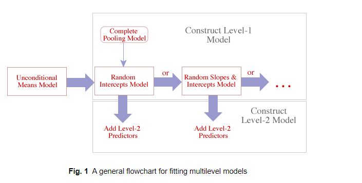

Schematic from Jack Weiss’s course site.

Pick the best of these, then add level-2 predictors (predictors that are constant within clusters).

Strategy outlined by:

Singer, J. D. and Willett, J. B. (2003) Applied Longitudinal Data Analysis: Modeling Change and Event Occurrence. (Oxford University Press, Oxford, UK).

Random intercepts versus random coefficient models

Although random intercepts models are common. . .

Schielzeth and Forstmeier (2009) suggest random slopes are usually appropriate for level-1 predictors (i.e., when x varies within a subject).

Maximal model

Attempt to make inference from a maximal model:

• Include all random slopes that you can for level 1 predictors
• Simplify as needed when encountering convergence problems.

Lots of debate on how best to approach model building/selection.

Dealing with statistical dependence

Induced correlation: random intercepts model

\[R_{ij} = \beta_0 + b_{0i}+ \beta_1NAP_{ij} + \beta_2Exposure_i + \epsilon_{ij}\]

Variance of \(R_{ij} = var(b_{0i}+\epsilon_{ij}) = var(b_{0i}) +var(\epsilon_{ij}) = \sigma^2_{b_{0}} + \sigma^2_\epsilon\)

Covariance (\(Y_{ij}, Y_{ij^\prime}) = \sigma^2_{b_{0}}\) (2 observations, same cluster [beach] since they share \(b_{0i}\))

Covariance (\(Y_{ij}, Y_{i^\prime j}) = 0\) (2 observations taken from 2 different clusters [beaches])

Intraclass correlation = Cor\((Y_{ij}, Y_{ij^\prime})\) = \(\frac{\sigma^2_{b_{0}}}{\sigma^2_{b_{0}}+\sigma^2_\epsilon} = 0.28\), correlation among observations taken from the same cluster.

Multiple random effects

Crossed random effects Year and PackID

model1 <- lmer(log(HRsize) ~ Season + StudyArea + DiffDTScaled + LFD*EVIScaled +
                 (1 | PackID) + (1 | Year),  REML=TRUE, data = HRData)

Different levels of correlation induced by (1 | PACKID) + (1 | Year)

• Two observations from same pack will be correlated due to sharing a “PackID” random effect
• Two observations from same year will be correlated due to sharing a random a “Year” effect.

R for demonstration!

Marginal Distribution

\[Y_{i} = X_{i}\beta + Z_ib + \epsilon_{i}\] \[\epsilon_i \sim N(0, \Sigma_i)\] \[b \sim N(0, D)\]

\[Y_i|b \sim N(X_i\beta+Z_ib, \Sigma_i)\] \[b \sim N(0, D)\]

If we average over (or integrate out) the random effects, we get the marginal Distribution of \(Y\).

\[Y_i \sim N(X_i\beta, V_i), V_i = Z_iDZ_i^\prime + \Sigma_i\]

This is the likelihood that R maximizes to get \(\hat{\beta}, \hat{D}, \hat{\Sigma_i}\).

Marginal likelihood

For random intercepts model:

\[Y_{i}\sim N(X_i\beta, V_i)\]

\(V_i = \begin{bmatrix} \sigma^2 & \rho & \cdots & \rho \\ \rho & \ddots & \ddots & \vdots \\ \vdots & \ddots & \ddots & \rho \\ \rho & \cdots & \rho & \sigma^2 \end{bmatrix}\) \(\rho = \frac{\sigma^2_{b_{0}}}{\sigma^2_{b_{0}}+\sigma^2_\epsilon}\)

Var/Cov matrix for \(Y\) (all data) = \(\begin{bmatrix} V_i & 0 & \cdots & 0 \\ 0 & \ddots & \ddots & \vdots \\ \vdots & \ddots & \ddots & 0 \\ 0 & \cdots & 0 & V_i \end{bmatrix}\)

Fitting the marginal model using gls

We might have posited this model directly.

We can fit it using the gls function in the nlme library

The gls function also allows for:

• A variety of assumptions for capturing within-subject correlation
  • ar(1) time series
  • Spatial covariance

• Methods for modeling heterogeneous variance
  • can allow the variance to differ by group (e.g., by exposure level)
  • can allow the variance to depend on a continuous predictor, \(x\) (e.g., var = \(\sigma^2 x^{2\theta}\))

See Ch 4 Zuur et al. and the section of the course on gls models.

Marginal Model fit using gls

gls.fit<-gls(Richness~NAPc+exposure.c, method="REML",
             correlation=corCompSymm(form=~1|Beach),
            data=RIKZdat)
summary(gls.fit)

Generalized least squares fit by REML
  Model: Richness ~ NAPc + exposure.c 
  Data: RIKZdat 
       AIC      BIC    logLik
  240.5538 249.2422 -115.2769

Correlation Structure: Compound symmetry
 Formula: ~1 | Beach 
 Parameter estimate(s):
      Rho 
0.2798938 

Coefficients:
                  Value Std.Error   t-value p-value
(Intercept)    3.170680 1.1739987  2.700752  0.0099
NAPc          -2.581708 0.4883901 -5.286160  0.0000
exposure.cLow  4.532777 1.5755610  2.876929  0.0063

 Correlation: 
              (Intr) NAPc  
NAPc          -0.028       
exposure.cLow -0.746  0.037

Standardized residuals:
       Min         Q1        Med         Q3        Max 
-1.5551728 -0.6415409 -0.1554932  0.4150315  3.3566242 

Residual standard error: 3.604905 
Degrees of freedom: 45 total; 42 residual