Correlated Data Overview

FW8051 Statistics for Ecologists

Learning Objectives

• Be able to model correlated binary and correlated count data using generalized linear mixed effect models (GLMMs) and generalized estimating equations (GEEs)

• Be able to interpret parameters in linear and generalized linear mixed effects models

• Be able to describe models and their assumptions using equations and text and match parameters in these equations to estimates in computer output.

Correlated Data Methods in Ecology

For data that are normally distributed:

• Linear mixed effects model
  
• Generalized Least Squares

For count or binary data:

• Generalized linear mixed effects models (GLMMS)
  
• Generalized Estimating Equations (GEE)

Fieberg, J., Rieger, R.H., Zicus, M. C., Schildcrout, J. S. 2009. Regression modelling of correlated data in ecology: subject specific and population averaged response patterns. Journal of Applied Ecology 46:1018-1025.

Mallard Nesting structures

Research Questions: which types of cylinders are best (single or double)?

Where should they be placed?

Mallard Data

• 110 nest structures placed in 104 wetlands
• Structure type (single versus double) was chosen randomly at each location
  • 53 single-cylinders, 57 double-cylinders
• Occupancy (0,1) and clutch sizes were recorded in 1997, 1998, 1999

Zicus, M.C., J. Fieberg and D. P. Rave. 2003. Does mallard clutch size vary with landscape composition: a different view. Wilson Bulletin 114:409-413.

Zicus, M. C., D. P. Rave, and J. Fieberg. 2006. Cost effectiveness of single- vs. double-cylinder over-water nest structures. Wildlife Society Bulletin 34:647-655.

Zicus, M. C., Rave, D. P., Das, A., Riggs, M. R., and Buitenwerf, M. L. (2006). Influence of land use on mallard nest‐structure occupancy. The Journal of wildlife management, 70(5), 1325-1333.

Example Clutch Size Data

\(Y_{ij}\) = clutch size for the \(i^{th}\) structure during year \(j\)

\(Init.Date_{ij}\) = nest initiation date (Julian day) for the \(i^{th}\) structure during year \(j\)

\(I(deply=2)_{i}\) = 0 if \(i^{th}\) structure is a single cylinder, 1 if double cylinder

Model: \[Y_{ij} \mid b_{0i} \sim N(\mu_{ij}, \sigma^2_{\epsilon})\] \[\mu_{ij} = (\beta_0 + b_{0i}) + \beta_1Init.Date_{ij} + \beta_2I(deply=2)_i\] \[b_{0i} \sim N(0, \sigma^2_{b_0})\]

Similar to including “structure” as a series of dummy variables with the added assumption that the parameters are drawn from a normal distribution

Generalized Least Squares

For normally distributed response data, we can fit correlated data models without having to resort to random effects:

\[Clutch size_{ij} = \beta_0 + \beta_1Init.Date_{ij}+ \beta_2I(deply=2)_i +\epsilon_{ij}\] \[\epsilon \sim N(0, \Omega)\]

\(\Omega\) = Var/Cov matrix for \(\epsilon\). We no longer assume the errors, \(\epsilon_{ij}\), are independent!

Generalized Least Squares

\[Clutch size_{ij} = \beta_0 + \beta_1Init.Date_{ij}+ \beta_2I(deply=2)_i+\epsilon_{ij}\]

\[\epsilon \sim N(0, \Omega)\]

Compound symmetric covariance matrix for within-cluster data:

\[\Omega= \begin{bmatrix} \Sigma_i & 0 & \cdots & 0 \\ 0 & \ddots & \ddots & \vdots \\ \vdots & \ddots & \ddots & 0 \\ 0 & \cdots & 0 & \Sigma_i \end{bmatrix} \text{ with } \Sigma_i = \begin{bmatrix} \sigma^2 & \rho\sigma^2 & \cdots & \rho \sigma^2 \\ \rho \sigma^2 & \ddots & \ddots & \vdots \\ \vdots & \ddots & \ddots & \rho \sigma^2 \\ \rho \sigma^2 & \cdots & \rho \sigma^2 & \sigma^2 \end{bmatrix}\]

Correlation between:

• 2 observations from the same cluster = \(\rho\)
• 2 observations taken from different clusters = \(0\)

This model is equivalent to a linear mixed effects model with random intercepts for each structure! Note: \(\rho = \frac{\sigma^2_{b_0}} {\sigma^2_{b_0}+ \sigma^2_{\epsilon}}\) and \(\sigma^2 = \sigma^2_{b_0}+ \sigma^2_{\epsilon}\).

Extensions to Count and Binary Data

Unlike the multivariate normal distribution, Poisson, Negative Binomial, Bernoulli, Binomial distributions

• Are NOT parameterized in terms of separate mean and variance parameters.

• Variance is a function of the mea7n
  • Poisson \(Var(Y|X) = E(Y|X)\)
  • Bernoulli \(Var(Y|X) = E(Y|X)(1-E(Y|X))\)

• Unlike the Normal distribution, there are no multivariate Poisson or Binomial analogs that allow correlation to be directly modeled

Extensions to Count and Binary Data

2 Options:

• Start with generalized linear models (logistic or Poisson regression) and add random coefficients (intercepts, slopes)
• Use generalized estimating equations or cluster-level bootstrap (recognizing clusters serve as independent units)

Option 1: Generalized linear mixed effects models

Generalized Linear Mixed Effects Models

Systematic component: \(g(\mu_{ij}) = \eta_{ij} = (\beta_0 + b_{0i}) + (\beta_1 + b_{1i})x_{ij}\)

Random components:

• \(Y_{ij} | b_{0i}, b_{1i} \sim f(y_{ij} | b_{0i}, b_{1i})\), with \(f(y_i | b_{0i}, b_{1i})\) in the exponential family (e.g., Poisson, binomial).
• \(b_{0i}\) and \(b_{1i}\) allow intercepts and parameters to vary among groups.
  
• Usually assume: (\(b_{0i}, b_{1i}) \sim N(0, \Sigma\))

Conditional models

Poisson-normal model:

• \(Y_{ij} | b_i \sim\) Poisson(\(\lambda_{ij}\))
• \(log(\lambda_{ij}) = (\beta_0 + b_{0i}) + (\beta_1 + b_{1i})x_{ij}\)
• (\(b_{0i}, b_{1i}) \sim N(0, \Sigma\))

Logistic-normal model:

• \(Y_{ij} | b_i \sim\) Bernoulli(\(p_{ij}\))
  
• \(logit(p_{ij}) = (\beta_0 + b_{0i}) + (\beta_1 + b_{1i})x_{ij}\)
• (\(b_{0i}, b_{1i}) \sim N(0, \Sigma\))

Frequentist analysis: the \(b\)’s are unobserved random variables…we do not estimate them! Rather, we estimate \(\beta_0, \beta_1, \Sigma\).

Non-linear models: Modeling Occupancy Probability

Logistic-normal model:

\[Y_{ij} | b_i \sim Bernoulli(p_{ij})\] \[\log[p_{ij}/(1-p_{ij})] = \beta_0 + b_{0i} + \beta_1VOM_{ij} + \beta_2I(deply=2)_i\] \[b_{0i} \sim N(0, \tau^2)\]

Structures have different “propensities” of being occupied:

• Depending on visual obstruction (VOM), structure type, and other unmeasured characteristics (\(b_{0i}\)) associated with the structure and the landscape in which it is placed.

Parameter Estimation

To estimate parameters using Maximum Likelihood, we need to determine:

• the distribution of \(Y\) (not \(Y|b_i\))

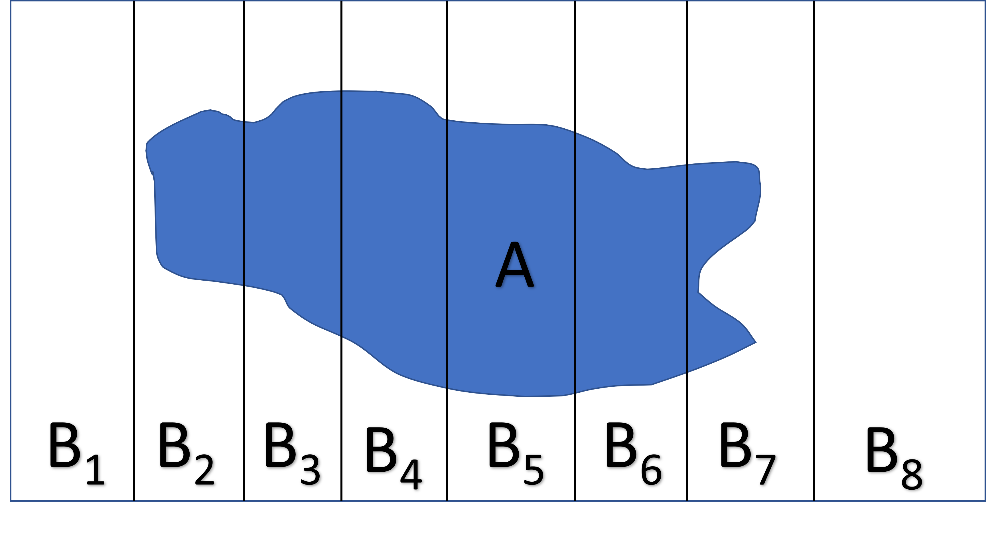
Total law of Probability If events \(B_1, B_2, \ldots, B_k\) are mutually exclusive and together make up all possibilities, then:

\(P(A) = \sum_iP(A|B_i)P(B)\)

Unconditional Model and Likelihood

To determine the distribution of \(Y_{ij}\), we integrate over the random effects:

\[L(Y_{ij} | \beta, \Sigma) = \int f(Y_{ij} | b_i)f(b_i)db_i\]

• \(\beta\) = fixed effects parameters in \(f(Y_{ij} | b_i)\)
• \(\Sigma\) are variance parameters of the random effects distribution, \(f(b_i)\)

Normally Distributed Data: Linear Mixed Effects Models

\[Y_{ij}|b \sim N(\mu_{ij}, \sigma^2)\] \[\mu_{ij} = X_{ij}\beta + Z_ib\] \[b \sim N(0, \Sigma)\]

If we average over (or integrate out) the random effects (\(b\)), we get the marginal distribution of \(Y\):

\[Y \sim MVN(X\beta, \Omega)\] \[\Omega = Z\Sigma Z^\prime + \sigma^2I\]

\[I= \begin{bmatrix} 1 & 0 & \cdots & 0 \\ 0 & \ddots & \ddots & \vdots \\ \vdots & \ddots & \ddots & 0 \\ 0 & \cdots & 0 & 1 \end{bmatrix}_{(n \times n)}\]

\[Y \sim MVN(X\beta, \Omega)\]

Random Intercept Model:

\[\Omega= \begin{bmatrix} \Sigma_i & 0 & \cdots & 0 \\ 0 & \ddots & \ddots & \vdots \\ \vdots & \ddots & \ddots & 0 \\ 0 & \cdots & 0 & \Sigma_i \end{bmatrix} \text{ with }\] \[\Sigma_i = \begin{bmatrix} \tau^2 + \sigma^2 & \tau^2 & \cdots & \tau^2 \\ \tau^2 & \ddots & \ddots & \vdots \\ \vdots & \ddots & \ddots & \tau^2 \\ \tau^2 & \cdots & \tau^2 & \tau^2 + \sigma^2 \end{bmatrix}\]

GLS Model with compound-symmetric correlation structure:

\[\Omega= \begin{bmatrix} \Sigma_i & 0 & \cdots & 0 \\ 0 & \ddots & \ddots & \vdots \\ \vdots & \ddots & \ddots & 0 \\ 0 & \cdots & 0 & \Sigma_i \end{bmatrix} \text{ with }\] \[\Sigma_i = \begin{bmatrix} \sigma^2 & \rho\sigma^2 & \cdots & \rho \sigma^2 \\ \rho \sigma^2 & \ddots & \ddots & \vdots \\ \vdots & \ddots & \ddots & \rho \sigma^2 \\ \rho \sigma^2 & \cdots & \rho \sigma^2 & \sigma^2 \end{bmatrix}\]

Logistic-normal random intercept model

\[Y_{ij} |b_i \sim Bernoulli(p_{ij})\] \[logit(p_{ij}) = \beta_0 + b_{0i} + \beta_{1}x_{ij}\] \[b_{0i} \sim N(0, \sigma^2_{b})\]

• \(f(Y_{ij} |b_i) = p_{ij}^{Y_{ij}}(1-p_{ij})^{1-Y_{ij}}\)
• \(f(b_i) = \frac{1}{\sqrt{2\pi}\sigma_{b}}e^{\frac{(b_{0i}-0)^2}{2\sigma^2_{b}}}\)

\[L(Y_{ij} | \beta, \Sigma) = \int f(Y_{ij} | b_i)f(b_i)db_i\]

\[\int \left[ \frac{exp(\beta_0 + b_{0i} + \beta_1x_{ij})}{1+exp(\beta_0 + b_{0i} + \beta_1x_{ij})}\right]^{Y_{ij}}\left[ \frac{1}{1+exp(\beta_0 + b_{0i} + \beta_1x_{ij})}\right]^{1-Y_{ij}} \frac{1}{\sqrt{2\pi}\sigma_{b}}e^{\frac{(b_{0i}-0)^2}{2\sigma^2_{b}}}db_{0i}\]

No closed-form solution!

Unconditional Model and Likelihood

How do we use maximum likelihood to estimate parameters?

\[L(Y_{ij} | \beta, \Sigma) = \prod_{i=1}^{n} \int f(Y_{ij} | b_i)f(b_i)db_i\]

Options:

• Approximate \(\prod_{i=1}^{n} \int f(Y_{ij} | b_i)f(b_i)\), then maximize
  
• Use numerical integration (can be slow, difficult, particularly with multiple random effects)
• Add priors, and use Bayesian techniques

Numerical Integration: glmer

nAGQ

• specifies number of points per axis for evaluating the adaptive Gauss-Hermite approximation to the log-likelihood.
• default = 1 (Laplace approximation)
• values > 1 produce greater accuracy in the evaluation of the log-likelihood at the expense of speed.
• a value of zero uses a faster but less exact form of parameter estimation for GLMMs (penalized iteratively reweighted least squares step).

See also mixed_model in the GLMMadaptive package.

LMEs versus GLMMs

Generalized linear mixed effects models are more challenging to fit than linear mixed effects models…and

Parameters in generalized linear mixed effects models have a “subject-specific”, but not “population-average” interpretation.

Parameter Interpretation: Linear mixed effects models

\[Clutch size_{ij} = (\beta_0 + b_{0i}) + \beta_1Init.Date_{ij} + \beta_2I(deply=2)_i+\epsilon_{ij}\] \[\epsilon_{ij} \sim N(0, \sigma^2)\] \[b_{0i} \sim N(0, \sigma^2_{b_0})\]

Assume \(\epsilon_{ij}\) and \(b_{0i}\) are independent.

How does clutch size vary with nest initiation date and structure type for a “typical” structure (i.e., one with \(b_{0i}\) = 0)?

• \(E[Y|X, b_{0i}=0] = \beta_0 + \beta_1Init.Date + \beta_2I(deply=2)\)

How does clutch size vary across the population of structures as a function of nest initiation date and structure type?

• \(E[Y|X] = \beta_0 + \beta_1Init.Date + \beta_2I(deply=2)\)

Fixed effects parameters have both population-averaged and subject-specific interpretations!

Parameter Interpretation: Generalized Linear Mixed Effects Models

\[Y_i | b_i \sim Bernoulli(p_i)\] \[\log[p_{ij}/(1-p_{ij})] = \beta_0 + b_{0i} + \beta_1VOM_{ij} + \beta_2I(deply=2)_i\] \[b_{0i} \sim N(0, \sigma^2_{b_0})\]

The fixed effects parameters in logistic regression models only have a subject-specific interpretation when we transform back to scales of interest!

• \(\exp(\beta_1)\) = change in the odds of occupancy as we increase VOM by 1 unit while holding and \(b_{0i}\) (i.e., “structure”) constant
• \(exp(\beta_2)\) = change in the odds of occupancy if we were to change a particular structure from a single to double cylinder model (and hold VOM constant)

Note: a subject-specific interpretation may not be meaningful for predictors that are constant within a cluster.

Interpretation of Parameters: GLMMS

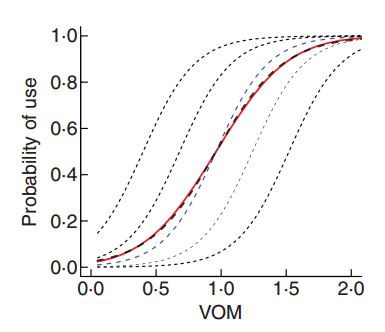
\(E[Y_{ij} | X]\) (red curve) is no longer the same as \(E[Y_{ij}|X, b_{0i}=0]\) (blue curve)!

GLMMs and Population-Average Response Patterns

\[Y_{ij} | b_{0i}, b_{1i} \sim f(y_{ij} | b_{0i}, b_{1i})\] \[(b_{0i}, b_{1i}) \sim N(0, \Sigma), \mbox{ with}\]

\(f(y_i | b_{0i}, b_{1i})\) given by Poisson, binomial, negative binomial.

How can we quantify how \(E[Y|X]\) changes with \(X\) (as opposed to \(E[Y |X, b_{0i}, b_{1i}]\) or \(E[Y |X, b_{0i}= b_{1i}=0]\))?

• Integrate (i.e. average) over the random effects using simulations: simulate several subject-specific response curves from the fitted model, transform back to the response scale, then average.
• Approximations in the literature for specific models (see Section 19 in book)
• mixed_model + marginal_coefs in GLMMadaptive package to estimate equivalent “marginal coefficients” (based on Hedeker et al. 2018).
  

Hedeker, D., du Toit, S. H., Demirtas, H. and Gibbons, R. D. (2018), A note on marginalization of regression parameters from mixed models of binary outcomes. Biometrics 74, 354-361.

GLMM Resources on Canvas

Readings:

• Bolker et al. 2008. Generalized linear mixed models: a practical guide for ecology and evolution
• Bolker et al. 2013: Strategies for fitting nonlinear ecological models in R, AD Model Builder, and BUGS

Useful Links

• GLMM wiki
• GLMMS worked examples
• GLMM FAQ

Option 2: Generalized Estimating equations

Generalized Estimating Equations

• Motivation (least squares, maximum likelihood…)
• Assumptions and implementation of GEE approach

Least Squares and Maximum Likelihood

For Normally distributed data:

\(L(\mu, \sigma^2; y_1, y_2, \ldots, y_n) = \prod_{i=1}^n \frac{1}{\sqrt{2\pi}\sigma}\exp\left(-\frac{(y_i-\mu)^2}{2\sigma^2}\right)\)

With linear regression, we assume \(Y_i \sim N(\mu_i, \sigma^2)\), with \(\mu_i = \beta_0 + X_i\beta_1\) so…

\(L(\beta_0, \beta_1, \sigma; x) = \prod_{i=1}^n \frac{1}{\sqrt{2\pi}\sigma}\exp\left(-\frac{(y_i-\beta_0+X_i\beta_1)^2}{2\sigma^2}\right) =\frac{1}{(\sqrt{2\pi}\sigma)^n}\exp\left(-\sum_{i=1}^n\frac{(y_i-\beta_0+X_i\beta_1)^2}{2\sigma^2}\right)\)

\(\Rightarrow logL =-nlog(\sigma) - \frac{n}{2}log(2\pi) -\sum_{i=1}^n\frac{(y_i-\beta_0+X_i\beta_1)^2}{2\sigma^2}\)

\(\Rightarrow\) maximizing logL \(\Rightarrow\) minimizing \(\sum_{i=1}^n\frac{(y_i-\beta_0+X_i\beta_1)^2}{2\sigma^2}\)

or, equivalently \(\sum_{i=1}^n(y_i-\beta_0-X_i\beta_1)^2\)

Least squares

\[\begin{gather} \sum_{i=1}^n (Y_i - E[Y_i|X_i])^2 \newline = \sum_{i=1}^n (Y_i - (\beta_0+X_{1i}\beta_1+\ldots))^2 \end{gather}\]

Least squares leads to the following set of equations for estimating parameters (take the derivative and set = 0):

\[2\sum_{i=1}^n \frac{\partial E[Y_i|X_i]}{\partial \beta}(Y_i -E[Y_i|X_i]) = 0\]

Generalized Linear Models

Maximum Likelihood estimators are found by solving:

\(\sum_{i=1}^n \frac{\partial E[Y_i|X_i]}{\partial \beta}V_i^{-1}(Y_i -E[Y_i|X_i]) = 0\).

Logistic Regression:

• \(E[Y_i|X_i]= \exp(X_i\beta)/[1+\exp(X_i\beta)]\)
• \(V_i = Var[Y_i|X_i]= E[Y_i|X_i](1-E[Y_i|X_i])\)

Poisson Regression:

• \(E[Y_i|X_i]= \exp(X_i\beta)\)
• \(V_i = Var[Y_i|X_i]= E[Y_i|X_i]\)

Generalized Estimating Equations (GEE)

GEE: \(\hat{\beta}\) solves: \(\sum_{i=1}^n \frac{\partial \mu_i}{\partial \beta}V_i(\alpha)^{-1}(Y_i -E[Y_i|X_i]) = 0\).

• Specify mean (\(E[Y|X]\)) and variance covariance matrix (\(V_i\)) of the data from each individual
• Write \(V_i(\alpha)\) in terms of variances and correlations among observations for each individual= \(A_i^{1/2}R_i(\alpha)A_i^{1/2}\)
  
• Determine the variance model based on the type of data (e.g., \(A_i = \phi E[Y|X]\) for count data, \(A_i = E[Y|X](1-E[Y|X])\) for binary data)

\(R_i\) = working correlation model that describes within subject correlation.

• Examples include exchangeable (equal correlation among all observations), Ar(1) (time series), unstructured

Generalized Estimating Equations (GEE)

GEE: \(\hat{\beta}\) solves: \(\sum_{i=1}^n \frac{\partial \mu_i}{\partial \beta}V_i(\alpha)^{-1}(Y_i -E[Y_i|X_i]) = 0\).

• Model the mean and variance as a function of explanatory variables (\(E(Y|X)\) and \(Var(Y|X)\))
• Make no other distributional assumptions (“quasi-likelihood”)
• Uses large sample theory for statistical inference, treating clusters as independent
• Fixed effects parameters have a population-averaged interpretation (how does \(y\) change across the population of structures that have different values of \(x\) )
• Fit using geeglm in geepack library

Theory

Estimates will be asymptotically unbiased (think “large number of clusters”)

• Even if the assumed variance & covariance models are wrong
• Better assumptions regarding the variance & correlation structure lead to more precise estimates
• Requires “missing data” to be missing completely at random (a simple way to think about this assumption is that the amount of data for each cluster is random)

Uses “robust” (or “sandwich”) standard errors, treating clusters as independent observational units

• \(\hat{\beta} \pm 1.96SE\) gives valid CIs (for large numbers of clusters)