Notes on Mid-term

FW8051 Statistics for Ecologists

Multiple Regression problem

lm.ref <- lm(log(lj_length) ~ log(skull_length)*Species, data = fishmorph2)

\[\log(\text{lower jaw length})_i \sim N(\mu_i, \sigma^2)\] \[\mu_i = \beta_0 + \beta_1\log(\text{Skull Length})_i + \beta_2I(Species=PL)_i + \beta_3I(Species=XA)_i +\] \[\beta_4\log(\text{Skull Length})_iI(Species=PL)_i+ \beta_5\log(\text{Skull Length})_iI(Species=XA)_i\]

\(\beta_0\) = mean or expected log(lower jaw length) when log(skull length) = 0 and species is AP (Anoplarchus purpurescens)
\(\beta_1\) = increase in the expected value of log lower jaw length as we increase log(skull length) by 1 when species is AP (Anoplarchus purpurescens)
\(\beta_2\) = difference in intercept for Species = PL relative to the intercept for species = AP; \((\beta_0 + \beta_2)\) gives the mean or expected log(lower jaw length) when log(skull length) = 0 and species is PL
\(\hat{\sigma}^2 = 0.0281^2\) tells us how much unexplained variability we have about the line.

Design matrix

For the final exam, make sure you can determine the design matrix this without the help of model.matrix.

newdata<-data.frame(Species = c("Anoplarchus_purpurescens", "Xiphister_atropurpureus"), 
                    skull_length = c(exp(2), exp(1.5)), lj_length = c(0, 0))
design<-model.matrix(lm.ref, data=newdata)
design[,]

  (Intercept) log(skull_length) SpeciesPholis_laeta
1           1               2.0                   0
2           1               1.5                   0
  SpeciesXiphister_atropurpureus log(skull_length):SpeciesPholis_laeta
1                              0                                     0
2                              1                                     0
  log(skull_length):SpeciesXiphister_atropurpureus
1                                              0.0
2                                              1.5

newdata<-data.frame(Species = c("Anoplarchus_purpurescens", "Xiphister_atropurpureus"), 
                    skull_length = c(exp(2), exp(1.5)), lj_length = c(0, 0))
design<-model.matrix(~Species*log(skull_length), data=newdata)
design[,]

  (Intercept) SpeciesXiphister_atropurpureus log(skull_length)
1           1                              0               2.0
2           1                              1               1.5
  SpeciesXiphister_atropurpureus:log(skull_length)
1                                              0.0
2                                              1.5

Means coding

lm.means <- lm(log(lj_length) ~ log(skull_length)*Species - log(skull_length) -1, data= fishmorph2)
summary(lm.means)


Call:
lm(formula = log(lj_length) ~ log(skull_length) * Species - log(skull_length) - 
    1, data = fishmorph2)

Residuals:
      Min        1Q    Median        3Q       Max 
-0.036489 -0.021110 -0.004249  0.022981  0.040137 

Coefficients:
                                                  Estimate Std. Error t value
SpeciesAnoplarchus_purpurescens                   -1.32633    0.12749 -10.403
SpeciesPholis_laeta                               -1.57038    0.28260  -5.557
SpeciesXiphister_atropurpureus                    -0.94076    0.09015 -10.435
log(skull_length):SpeciesAnoplarchus_purpurescens  1.39942    0.05740  24.380
log(skull_length):SpeciesPholis_laeta              1.39505    0.13760  10.139
log(skull_length):SpeciesXiphister_atropurpureus   1.11998    0.03815  29.360
                                                  Pr(>|t|)    
SpeciesAnoplarchus_purpurescens                   2.96e-08 ***
SpeciesPholis_laeta                               5.49e-05 ***
SpeciesXiphister_atropurpureus                    2.84e-08 ***
log(skull_length):SpeciesAnoplarchus_purpurescens 1.76e-13 ***
log(skull_length):SpeciesPholis_laeta             4.17e-08 ***
log(skull_length):SpeciesXiphister_atropurpureus  1.14e-14 ***
---
Signif. codes:  0 '***' 0.001 '**' 0.01 '*' 0.05 '.' 0.1 ' ' 1

Residual standard error: 0.0281 on 15 degrees of freedom
Multiple R-squared:  0.9998,    Adjusted R-squared:  0.9997 
F-statistic: 1.273e+04 on 6 and 15 DF,  p-value: < 2.2e-16

Hypothesis tests

confint(lm.means)

                                                      2.5 %     97.5 %
SpeciesAnoplarchus_purpurescens                   -1.598064 -1.0545893
SpeciesPholis_laeta                               -2.172736 -0.9680278
SpeciesXiphister_atropurpureus                    -1.132916 -0.7486064
log(skull_length):SpeciesAnoplarchus_purpurescens  1.277071  1.5217612
log(skull_length):SpeciesPholis_laeta              1.101771  1.6883305
log(skull_length):SpeciesXiphister_atropurpureus   1.038671  1.2012844

If you used reference coding, then you need to use matrix multiplication (or a package like emmeans) to get the species-specific estimates and their uncertainty.

need to account for the variance of each parameter
and how parameters co-vary

See Section 3.12 in the book and also the GLS slides/application.

Non-linear regression

copepod <- copepod |> mutate(Temp25 = ifelse(Temp < 25, 0, Temp-25))
lm.linsp <- lm(Oxygen ~ Temp + Temp25, data = copepod)

effectplot<- ggeffects::ggpredict(lm.linsp, "Temp")
plot(effectplot, show_residuals = TRUE)

copepod$lm.linsp <- predict(lm.linsp)
ggplot(copepod, aes(x = Temp, y = Oxygen)) + 
  geom_point(alpha = 0.5) + # Using the data already in copepod.preds
  geom_line(aes(y = lm.linsp), linewidth = 1) +
  theme_bw() +labs(y = expression(Oxygen~Consumption~(mu*g~O[2]/mg/hr)),
       x = "Temperature (°C)")

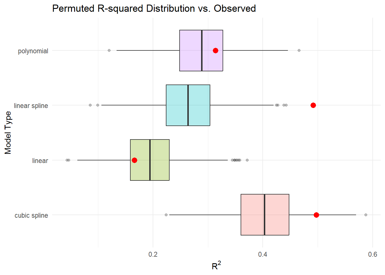
Out-of-sample \(R^2\)

We might expect out-of-sample \(R^2\) to be smaller than in-sample \(R^2\) if we use the data to inform our model in key ways:

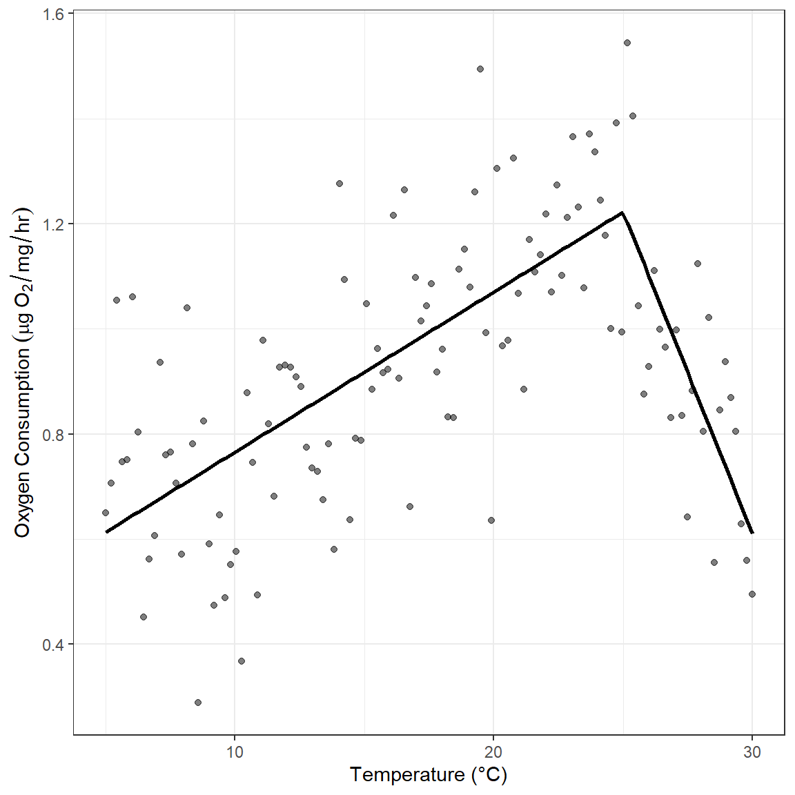
pick the location of a knot for the linear spline
determine how many df to allocate to cubic splines
decide on a quadratic or cubic polynomial

This problem was not perfect, because ideally we would like to replicate the full process of:

Collect a data set
Use the data to inform our model
Evaluate how the data-informed model performs on a new data set.

We didn’t replicate 1 and 2 (but replicated 3). But…